library(AutoScore)
data("sample_data")
names(sample_data)[names(sample_data) == "Mortality_inpatient"] <- "label"
check_data(sample_data)
Data type check passed. No NA in data. AutoScore on binary outcomes is the original form of the AutoScore, implemented by five functions: AutoScore_rank(), AutoScore_Ordinal(), AutoScore_weighting(), AutoScore_fine_tuning() and AutoScore_testing().
In this chapter, we demonstrate the use of AutoScore to develop sparse risk scores for binary outcome, adjust parameters to improve interpretability, assess the performance of the final model and map the score to predict risks for new data. To facilitate clinical applications, in the following sections we have three demos for AutoScore Implementation with large and small dataset, as well as with missing data.
Citation for original AutoScore:
In Demo 1, we demonstrate the use of AutoScore on a dataset with 20,000 observations using split-sample approach (i.e., to randomly divide the full dataset into training, validation and test sets) for model development.
Load package and data
library(AutoScore)
data("sample_data")
names(sample_data)[names(sample_data) == "Mortality_inpatient"] <- "label"
check_data(sample_data)Data type check passed. No NA in data. Prepare training, validation, and test datasets
strat_by_label = FALSE, default) into training, validation, and test datasets (70%, 10%, 20%, respectively).strat_by_label = FALSE to stratify by label when splitting data.set.seed(4)
out_split <- split_data(data = sample_data, ratio = c(0.7, 0.1, 0.2),
strat_by_label = FALSE)
train_set <- out_split$train_set
validation_set <- out_split$validation_set
test_set <- out_split$test_setAutoScore Module 1
method: "rf" (default) or "auc".rf: random forest-based ranking.ntree: Number of trees required only when method = "rf" (Default: 100).ranking <- AutoScore_rank(train_set = train_set, method = "rf", ntree = 100)The ranking based on variable importance was shown below for each variable:
Age Lab_H Lab_K Lab_B Vital_E Vital_A Lab_I Lab_A
152.24380 151.60648 147.96133 134.85962 130.84508 128.05477 106.01727 96.68171
Vital_C Vital_B Lab_M Lab_J Vital_D Lab_D Vital_F Lab_E
94.91108 94.41436 92.31222 84.42058 83.63048 80.23488 77.07122 75.73559
Lab_C Lab_F Lab_L Lab_G Vital_G
75.48998 75.08788 72.61001 56.33592 56.08578 ![]()
auc: AUC-based ranking. Univariable models will be built based on the train set, and variables are ranked based on the AUC performance of corresponding univariable models on the validation set (validation_set).validation_set: validation set required only when method = "auc".ranking <- AutoScore_rank(train_set = train_set, method = "auc",
validation_set = validation_set)The auc-based ranking based on variable importance was shown below for each variable:
Lab_H Age Lab_B Lab_K Vital_E Vital_A Lab_M Lab_C
0.7016120 0.6926165 0.6796975 0.6741446 0.6708401 0.6319503 0.6010980 0.6010525
Lab_G Vital_C Vital_D Lab_F Lab_L Lab_A Vital_F Vital_G
0.5777848 0.5743282 0.5617414 0.5606434 0.5427415 0.5392167 0.5380191 0.5345188
Vital_B Lab_D Lab_I Lab_E Lab_J
0.5326130 0.5186835 0.5139225 0.4888609 0.4845179 ![]()
AutoScore Modules 2+3+4
n_min: Minimum number of selected variables (Default: 1).n_max: Maximum number of selected variables (Default: 20).categorize: Methods for categorizing continuous variables. Options include "quantile" or "kmeans" (Default: "quantile").quantiles: Predefined quantiles to convert continuous variables to categorical ones. (Default: c(0, 0.05, 0.2, 0.8, 0.95, 1)) Available if categorize = "quantile".max_cluster: The maximum number of cluster (Default: 5). Available if categorize = "kmeans".max_score: Maximum total score (Default: 100).auc_lim_min: Minimum y_axis limit in the parsimony plot (Default: 0.5).auc_lim_max: Maximum y_axis limit in the parsimony plot (Default: “adaptive”).AUC <- AutoScore_parsimony(
train_set = train_set, validation_set = validation_set,
rank = ranking, max_score = 100, n_min = 1, n_max = 20,
categorize = "quantile", quantiles = c(0, 0.05, 0.2, 0.8, 0.95, 1),
auc_lim_min = 0.5, auc_lim_max = "adaptive"
)Select 1 Variable(s): Area under the curve: 0.6649
Select 2 Variable(s): Area under the curve: 0.7466
Select 3 Variable(s): Area under the curve: 0.7729
Select 4 Variable(s): Area under the curve: 0.7915
Select 5 Variable(s): Area under the curve: 0.8138
Select 6 Variable(s): Area under the curve: 0.8268
Select 7 Variable(s): Area under the curve: 0.822
Select 8 Variable(s): Area under the curve: 0.8196
Select 9 Variable(s): Area under the curve: 0.8188
Select 10 Variable(s): Area under the curve: 0.8184
Select 11 Variable(s): Area under the curve: 0.8178
Select 12 Variable(s): Area under the curve: 0.8238
Select 13 Variable(s): Area under the curve: 0.8224
Select 14 Variable(s): Area under the curve: 0.8256
Select 15 Variable(s): Area under the curve: 0.8301
Select 16 Variable(s): Area under the curve: 0.8278
Select 17 Variable(s): Area under the curve: 0.8269
Select 18 Variable(s): Area under the curve: 0.8273
Select 19 Variable(s): Area under the curve: 0.8244
Select 20 Variable(s): Area under the curve: 0.8259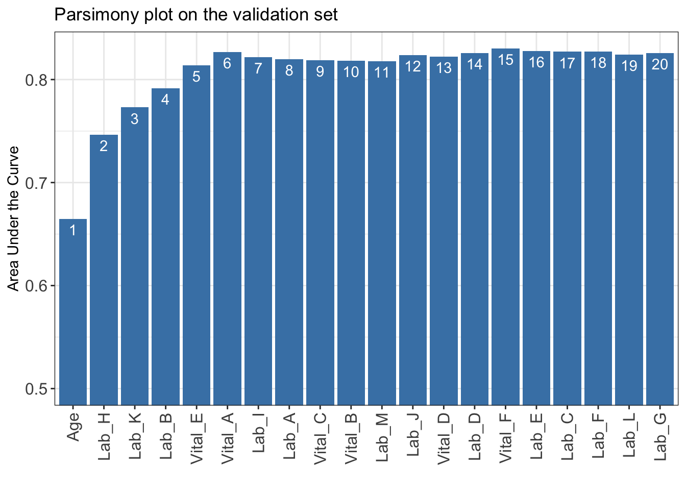
AUC for further analysis or export it to CSV to other software for plotting.write.csv(data.frame(AUC), file = "AUC.csv")num_var) based on the parsimony plot obtained in STEP(ii).num_var variables in the ranked list ranking obtained in STEP(i).final_variables based on the clinical preferences and knowledge.# Example 1: Top 6 variables are selected
num_var <- 6
final_variables <- names(ranking[1:num_var])
# Example 2: Top 9 variables are selected
num_var <- 9
final_variables <- names(ranking[1:num_var])
# Example 3: Top 6 variables, the 9th and 10th variable are selected
num_var <- 6
final_variables <- names(ranking[c(1:num_var, 9, 10)])Re-run AutoScore Modules 2+3
cut_vec with current cutoffs of continuous variables, which can be fine-tuned in STEP(iv).cut_vec <- AutoScore_weighting(
train_set = train_set, validation_set = validation_set,
final_variables = final_variables, max_score = 100,
categorize = "quantile", quantiles = c(0, 0.05, 0.2, 0.8, 0.95, 1)
)****Included Variables:
variable_name
1 Age
2 Lab_H
3 Lab_K
4 Lab_B
5 Vital_E
6 Vital_A
****Initial Scores:
======== ========== =====
variable interval point
======== ========== =====
Age <35 0
[35,49) 7
[49,76) 17
[76,89) 23
>=89 27
Lab_H <0.2 0
[0.2,1.1) 4
[1.1,3.1) 9
[3.1,4) 15
>=4 18
Lab_K <8 0
[8,42) 6
[42,58) 11
>=58 14
Lab_B <8.5 0
[8.5,11.2) 4
[11.2,17) 7
[17,19.8) 10
>=19.8 12
Vital_E <12 0
[12,15) 2
[15,22) 7
[22,25) 12
>=25 15
Vital_A <60 0
[60,73) 1
[73,98) 6
[98,111) 10
>=111 13
======== ========== =====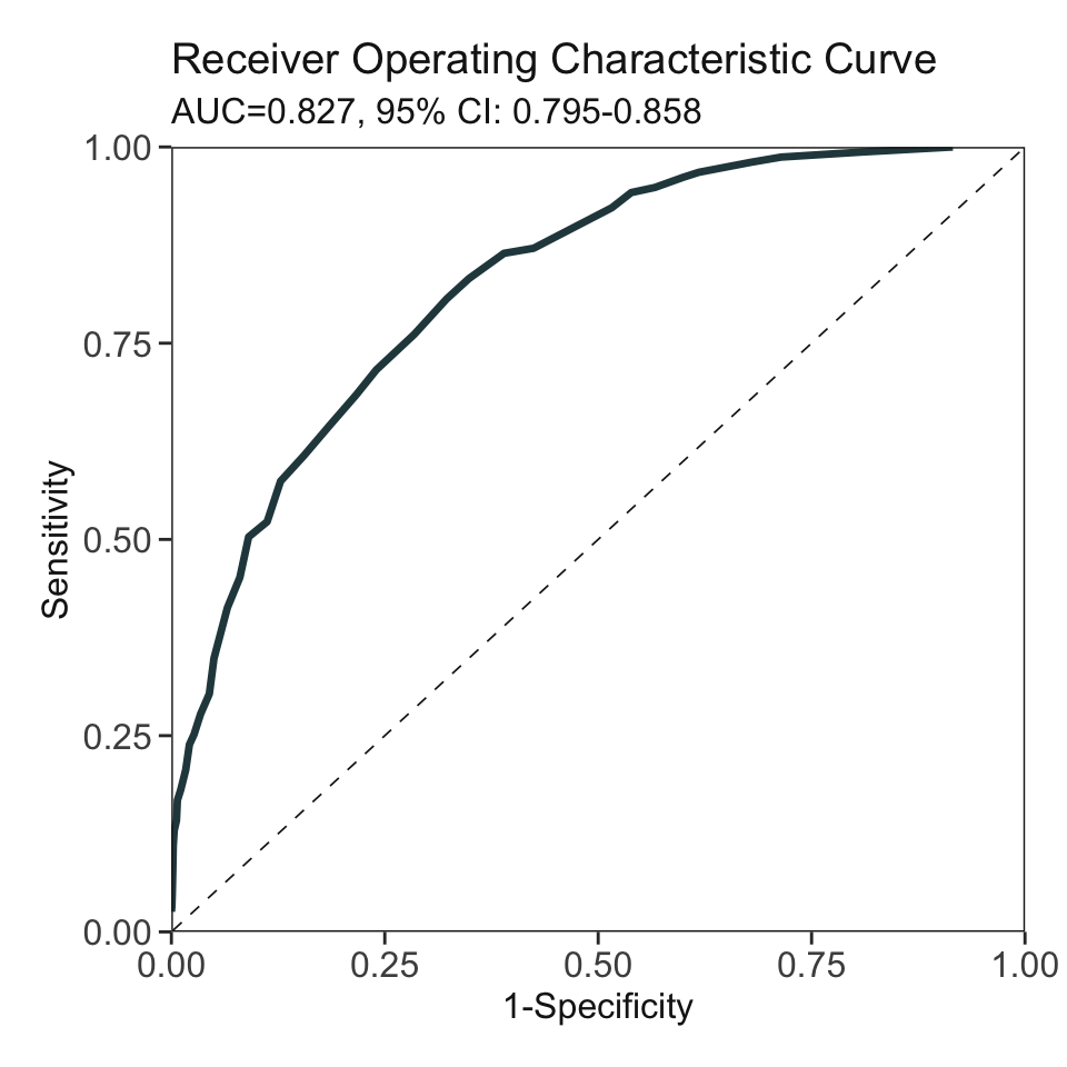
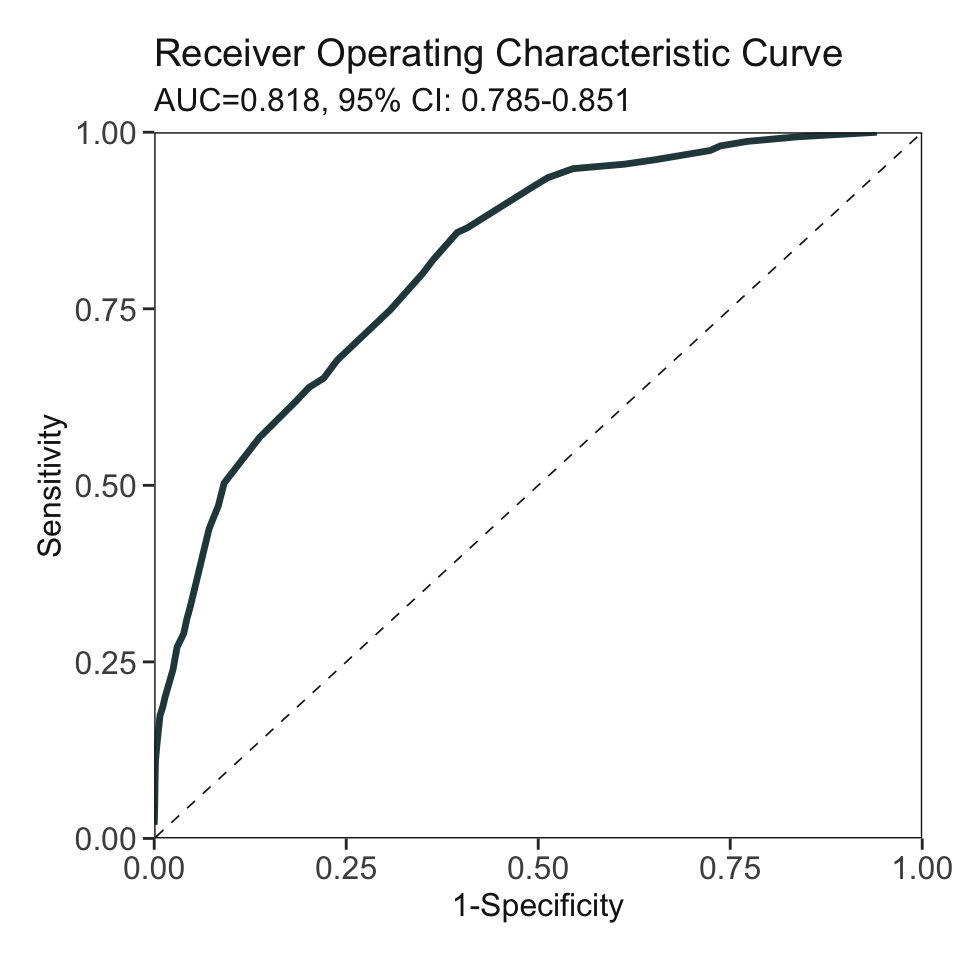
***Performance (based on validation set):
AUC: 0.8268 95% CI: 0.7953-0.8583 (DeLong)
Best score threshold: >= 57
Other performance indicators based on this score threshold:
Sensitivity: 0.8065
Specificity: 0.6775
PPV: 0.1736
NPV: 0.9766
***The cutoffs of each variable generated by the AutoScore are saved in cut_vec. You can decide whether to revise or fine-tune them AutoScore Module 5 & Re-run AutoScore Modules 2+3
cut_vec with domain knowledge to update the scoring table (AutoScore Module 5).## For example, we have current cutoffs of continuous variable: Age
## ============== =========== =====
## variable interval point
## ============== =========== =====
## Age <35 0
## [35,49) 7
## [49,76) 17
## [76,89) 23
## >=89 27 c(35, 49, 76, 89). We can fine tune the cutoffs as follows:# Example 1: rounding up to a nice number
cut_vec$Age <- c(35, 50, 75, 90)
# Example 2: changing cutoffs according to clinical knowledge or preference
cut_vec$Age <- c(25, 50, 75, 90)
# Example 3: combining categories
cut_vec$Age <- c(50, 75, 90)cut_vec$Lab_H <- c(0.2, 1, 3, 4)
cut_vec$Lab_K <- c(10, 40)
cut_vec$Lab_B <- c(10, 17)
cut_vec$Vital_A <- c(70, 98)
scoring_table <- AutoScore_fine_tuning(
train_set = train_set, validation_set = validation_set,
final_variables = final_variables, cut_vec = cut_vec, max_score = 100
)***Fine-tuned Scores:
======== ======== =====
variable interval point
======== ======== =====
Age <50 0
[50,75) 12
[75,90) 19
>=90 24
Lab_H <0.2 0
[0.2,1) 6
[1,3) 11
[3,4) 18
>=4 22
Lab_K <10 0
[10,40) 8
>=40 15
Lab_B <10 0
[10,17) 3
>=17 8
Vital_E <12 0
[12,15) 1
[15,22) 8
[22,25) 15
>=25 18
Vital_A <70 0
[70,98) 7
>=98 13
======== ======== =====
***Performance (based on validation set, after fine-tuning):
AUC: 0.8188 95% CI: 0.7862-0.8515 (DeLong)
Best score threshold: >= 55
Other performance indicators based on this score threshold:
Sensitivity: 0.8452
Specificity: 0.6336
PPV: 0.1623
NPV: 0.9799AutoScore Module 6
threshold: Score threshold for the ROC analysis to generate sensitivity, specificity, etc. If set to "best", the optimal threshold will be calculated (Default: "best").with_label: Set to TRUE if there are labels in the test_set and performance will be evaluated accordingly (Default: TRUE).with_label to FALSE if there are not label in the test_set and the final predicted scores will be the output without performance evaluation.pred_score <- AutoScore_testing(
test_set = test_set, final_variables = final_variables, cut_vec = cut_vec,
scoring_table = scoring_table, threshold = "best", with_label = TRUE
)
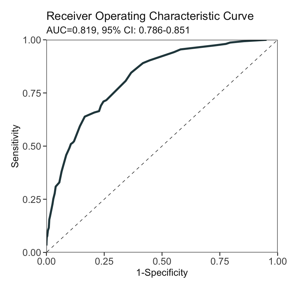
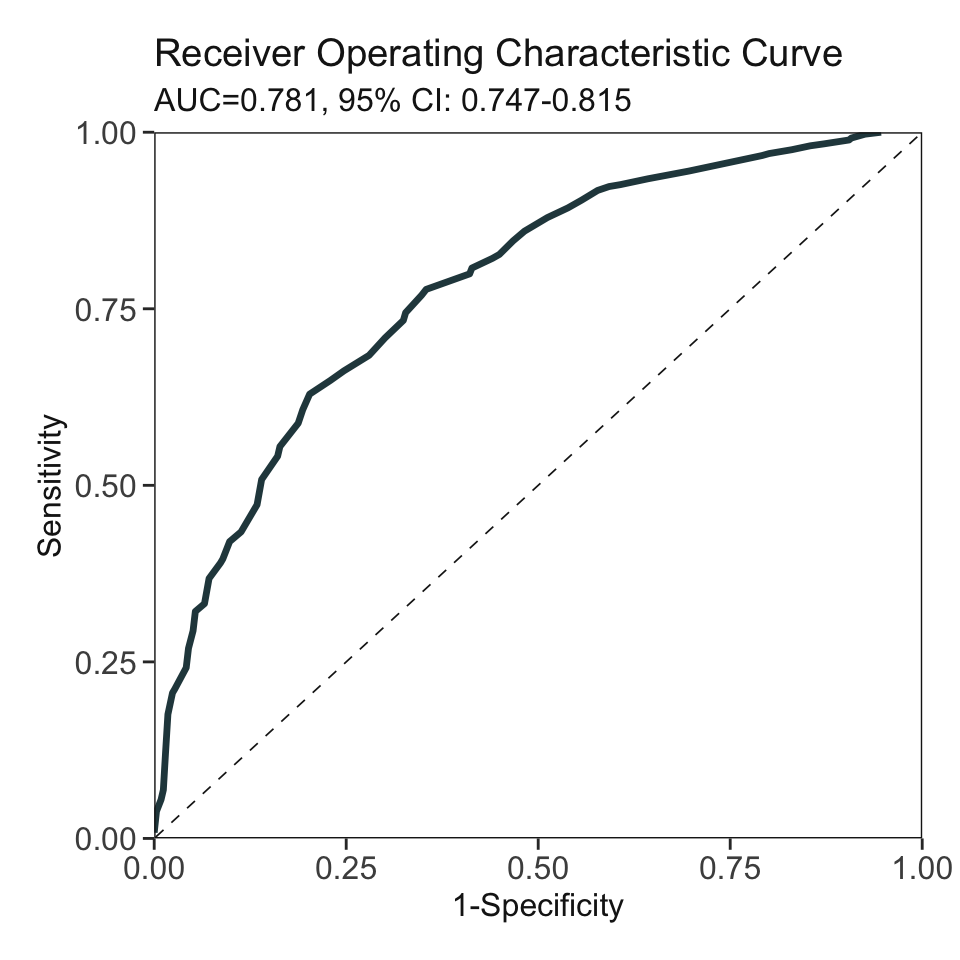
***Performance using AutoScore:
AUC: 0.8337 95% CI: 0.8125-0.8548 (DeLong)
Best score threshold: >= 59
Other performance indicators based on this score threshold:
Sensitivity: 0.7524 95% CI: 0.7003-0.8013
Specificity: 0.7652 95% CI: 0.7525-0.7788
PPV: 0.2106 95% CI: 0.1957-0.2249
NPV: 0.9739 95% CI: 0.9686-0.9789head(pred_score) pred_score Label
1 19 FALSE
2 41 FALSE
3 74 TRUE
4 37 FALSE
5 49 FALSE
6 34 FALSEprint_roc_performance() to generate the performance under different score thresholds (e.g., 50).print_roc_performance(pred_score$Label, pred_score$pred_score, threshold = 50)AUC: 0.8337 95% CI: 0.8125-0.8548 (DeLong)
Score threshold: >= 50
Other performance indicators based on this score threshold:
Sensitivity: 0.9055
Specificity: 0.5532
PPV: 0.1442
NPV: 0.986Further analysis to map score to risk (e.g., conversion table, model calibration, output the score).
conversion_table() to generate the performance under different risk (i.e., probability of mortality based on logistic regression estimation) cut-off (e.g., 0.01, 0.05, 0.1, 0.2, 0.5).conversion_table(pred_score = pred_score,
by = "risk", values = c(0.01, 0.05, 0.1, 0.2, 0.5))| Predicted Risk [>=] | Score cut-off [>=] | Percentage of patients (%) | Accuracy (95% CI) | Sensitivity (95% CI) | Specificity (95% CI) | PPV (95% CI) | NPV (95% CI) |
|---|---|---|---|---|---|---|---|
| 1% | 38 | 82 | 25.8% (24.5-27.1%) | 99% (97.7-100%) | 19.7% (18.4-21.1%) | 9.3% (9.1-9.5%) | 99.6% (99-100%) |
| 5% | 54 | 42 | 63.6% (62-64.9%) | 87% (83.1-90.6%) | 61.6% (60-63.1%) | 15.9% (15.1-16.6%) | 98.3% (97.8-98.7%) |
| 10% | 61 | 25 | 78.2% (77-79.4%) | 72% (67.1-76.5%) | 78.7% (77.4-80%) | 21.9% (20.4-23.6%) | 97.1% (96.7-97.6%) |
| 20% | 68 | 11 | 88% (87.1-88.9%) | 45% (39.1-50.5%) | 91.6% (90.7-92.4%) | 30.8% (27.4-34.3%) | 95.2% (94.8-95.7%) |
| 50% | 81 | 1 | 92.5% (92.2-92.9%) | 11.1% (7.8-14.7%) | 99.4% (99-99.6%) | 58% (45.6-70.6%) | 93.1% (92.8-93.3%) |
conversion_table() to generate the performance under different score thresholds (e.g., 20, 40, 60, 75).conversion_table(pred_score = pred_score,
by = "score", values = c(20,40,60,75))| Score cut-off [>=] | Predicted Risk [>=] | Percentage of patients (%) | Accuracy (95% CI) | Sensitivity (95% CI) | Specificity (95% CI) | PPV (95% CI) | NPV (95% CI) |
|---|---|---|---|---|---|---|---|
| 20 | 0.1% | 99 | 8.6% (8.3-8.9%) | 100% (100-100%) | 1% (0.7-1.4%) | 7.7% (7.7-7.8%) | 100% (100-100%) |
| 40 | 1.2% | 79 | 28.7% (27.4-30%) | 99% (97.7-100%) | 22.8% (21.5-24.2%) | 9.6% (9.5-9.8%) | 99.7% (99.2-100%) |
| 60 | 9.7% | 26 | 77.2% (75.9-78.5%) | 73.6% (68.7-78.2%) | 77.5% (76.1-78.8%) | 21.4% (19.9-22.9%) | 97.3% (96.7-97.7%) |
| 75 | 34.8% | 4 | 91.8% (91.2-92.3%) | 21.8% (17.3-26.7%) | 97.6% (97.1-98.1%) | 43.1% (35.8-50%) | 93.8% (93.4-94.1%) |
plot_predicted_risk(pred_score = pred_score, max_score = 100,
final_variables = final_variables,
scoring_table = scoring_table, point_size = 1)pred_score for further analysis or export it to CSV to other software (e.g., generating the calibration curve).write.csv(pred_score, file = "pred_score.csv")In Demo 2, we demonstrate the use of AutoScore on a smaller dataset where there are no sufficient samples to form a separate training and validation dataset. Thus, the cross validation is employed to generate the parsimony plot.
Load small dataset with 1000 samples
data("sample_data_small")Prepare training and test datasets
train_set is equal to validation_set and the ratio of validation_set should be 0. Then cross-validation will be implemented in the STEP(ii) AutoScore_parsimony().set.seed(4)
out_split <- split_data(data = sample_data_small, ratio = c(0.7, 0, 0.3),
cross_validation = TRUE)
train_set <- out_split$train_set
validation_set <- out_split$validation_set
test_set <- out_split$test_setAutoScore Module 1
method: "rf" (default) or "auc".rf: random forest-based ranking.ntree: Number of trees required only when method = "rf" (Default: 100).ranking <- AutoScore_rank(train_set = train_set, method = "rf", ntree = 100)The ranking based on variable importance was shown below for each variable:
Age Lab_B Lab_H Vital_E Lab_K Vital_A Lab_I Lab_J
37.406648 31.315285 25.564054 21.855069 20.907522 20.645694 16.788696 16.094679
Vital_B Lab_A Lab_M Vital_C Vital_F Lab_D Lab_C Lab_E
15.574365 14.651987 14.297510 13.765633 12.932043 12.679113 12.295000 12.165724
Lab_F Vital_D Lab_L Lab_G Vital_G
11.649415 11.431833 10.108408 9.297786 7.680821 ![]()
auc: AUC-based ranking. Univariable models will be built based on the train set, and variables are ranked based on the AUC performance of corresponding univariable models on the validation set (validation_set).validation_set: validation set required only when method = "auc".ranking <- AutoScore_rank(train_set = train_set, method = "auc",
validation_set = validation_set)The auc-based ranking based on variable importance was shown below for each variable:
Lab_B Age Vital_E Lab_H Lab_K Lab_C Vital_A Lab_G
0.6668343 0.6619857 0.6522559 0.6469780 0.6347585 0.6064601 0.5986108 0.5678392
Lab_A Lab_M Lab_F Vital_C Vital_D Lab_D Vital_B Lab_I
0.5672668 0.5614125 0.5613635 0.5613553 0.5500025 0.5469036 0.5395408 0.5288666
Vital_F Vital_G Lab_L Lab_E Lab_J
0.5207802 0.5175751 0.5124730 0.5098729 0.5059606 ![]()
AutoScore Modules 2+3+4
n_min: Minimum number of selected variables (Default: 1).n_max: Maximum number of selected variables (Default: 20).categorize: Methods for categorizing continuous variables. Options include "quantile" or "kmeans" (Default: "quantile").quantiles: Predefined quantiles to convert continuous variables to categorical ones. (Default: c(0, 0.05, 0.2, 0.8, 0.95, 1)) Available if categorize = "quantile".max_cluster: The maximum number of cluster (Default: 5). Available if categorize = "kmeans".max_score: Maximum total score (Default: 100).auc_lim_min: Minimum y_axis limit in the parsimony plot (Default: 0.5).auc_lim_max: Maximum y_axis limit in the parsimony plot (Default: “adaptive”).cross_validation: TRUE if cross-validation is needed, especially for small datasets.fold: The number of folds used in cross validation (Default: 10). Available if cross_validation = TRUE.do_trace: If set to TRUE, all results based on each fold of cross-validation would be printed out and plotted (Default: FALSE). Available if cross_validation = TRUE.AUC <- AutoScore_parsimony(
train_set = train_set, validation_set = validation_set,
rank = ranking, max_score = 100, n_min = 1, n_max = 20,
categorize = "quantile", quantiles = c(0, 0.25, 0.5, 0.75, 1),
auc_lim_min = 0.5, auc_lim_max = "adaptive",
cross_validation = TRUE, fold = 10, do_trace = FALSE
)***list of final mean AUC values through cross-validation are shown below
auc_set.sum
1 0.6332124
2 0.7254603
3 0.7381319
4 0.7623322
5 0.7695922
6 0.7735329
7 0.7728111
8 0.7700531
9 0.7665829
10 0.7634048
11 0.7651904
12 0.7617113
13 0.7571203
14 0.7694130
15 0.7650977
16 0.7572382
17 0.7603713
18 0.7650728
19 0.7656964
20 0.7645128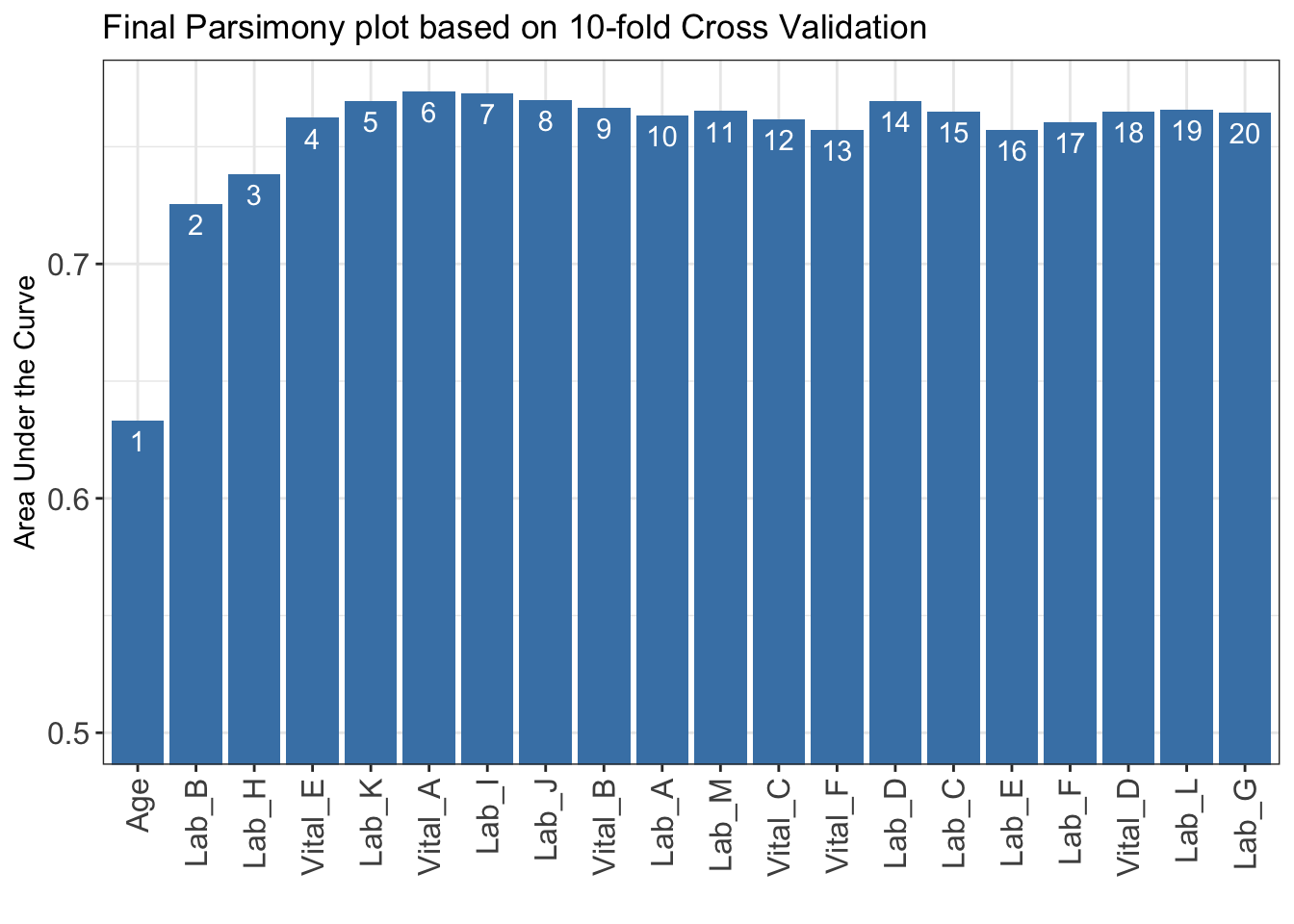
AUC for further analysis or export it to CSV to other software for plotting.write.csv(data.frame(AUC), file = "AUC.csv")num_var) based on the parsimony plot obtained in STEP(ii).num_var variables in the ranked list ranking obtained in STEP(i).final_variables based on the clinical preferences and knowledge.# Example 1: Top 6 variables are selected
num_var <- 6
final_variables <- names(ranking[1:num_var])
# Example 2: Top 9 variables are selected
num_var <- 9
final_variables <- names(ranking[1:num_var])
# Example 3: Top 6 variables, the 9th and 10th variable are selected
num_var <- 6
final_variables <- names(ranking[c(1:num_var, 9, 10)])Re-run AutoScore Modules 2+3
cut_vec with current cutoffs of continuous variables, which can be fine-tuned in STEP(iv).cut_vec <- AutoScore_weighting(
train_set = train_set, validation_set = validation_set,
final_variables = final_variables, max_score = 100,
categorize = "quantile", quantiles = c(0, 0.25, 0.5, 0.75, 1)
)****Included Variables:
variable_name
1 Age
2 Lab_B
3 Lab_H
4 Vital_E
5 Lab_K
****Initial Scores:
======== =========== =====
variable interval point
======== =========== =====
Age <52 0
[52,62) 15
[62,73) 21
>=73 30
Lab_B <11.9 0
[11.9,14.3) 9
[14.3,16.7) 15
>=16.7 21
Lab_H <1.2 0
[1.2,2.1) 15
[2.1,2.82) 13
>=2.82 19
Vital_E <16 0
[16,19) 4
[19,21) 9
>=21 19
Lab_K <13 2
[13,26) 0
[26,40) 4
>=40 11
======== =========== =====
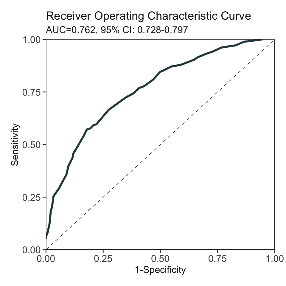
***Performance (based on validation set):
AUC: 0.781 95% CI: 0.7473-0.8148 (DeLong)
Best score threshold: >= 58
Other performance indicators based on this score threshold:
Sensitivity: 0.6291
Specificity: 0.7976
PPV: 0.771
NPV: 0.665
***The cutoffs of each variable generated by the AutoScore are saved in cut_vec. You can decide whether to revise or fine-tune them AutoScore Module 5 & Re-run AutoScore Modules 2+3
cut_vec with domain knowledge to update the scoring table (AutoScore Module 5).## For example, we have current cutoffs of continuous variable:
## ============== =========== =====
## variable interval point
## ============== =========== =====
#> Lab_K <9 0
#> [9,43.2) 1
#> [43.2,59) 9
#> >=59 13 c(9, 43.2, 59). We can fine tune the cutoffs as follows:# Example 1: rounding up to a nice number
cut_vec$Lab_K <- c(9, 45, 60)
# Example 2: changing cutoffs according to clinical knowledge or preference
cut_vec$Lab_K <- c(15, 45, 60)
# Example 3: combining categories
cut_vec$Lab_K <- c(45, 60)cut_vec$Lab_H <- c(1, 2, 3)
cut_vec$Age <- c(35, 50, 80)
cut_vec$Lab_B <- c(8, 12, 18)
cut_vec$Vital_E <- c(15, 22)
scoring_table <- AutoScore_fine_tuning(
train_set = train_set, validation_set = validation_set,
final_variables = final_variables, cut_vec = cut_vec, max_score = 100
)***Fine-tuned Scores:
======== ======== =====
variable interval point
======== ======== =====
Age <35 0
[35,50) 2
[50,80) 18
>=80 23
Lab_B <8 0
[8,12) 8
[12,18) 15
>=18 22
Lab_H <1 0
[1,2) 12
[2,3) 13
>=3 18
Vital_E <15 0
[15,22) 10
>=22 20
Lab_K <45 0
[45,60) 10
>=60 17
======== ======== =====
***Performance (based on validation set, after fine-tuning):
AUC: 0.7623 95% CI: 0.7275-0.7971 (DeLong)
Best score threshold: >= 60
Other performance indicators based on this score threshold:
Sensitivity: 0.5714
Specificity: 0.8214
PPV: 0.7761
NPV: 0.6389AutoScore Module 6
threshold: Score threshold for the ROC analysis to generate sensitivity, specificity, etc. If set to "best", the optimal threshold will be calculated (Default: "best").with_label: Set to TRUE if there are labels in the test_set and performance will be evaluated accordingly (Default: TRUE).with_label to FALSE if there are not label in the test_set and the final predicted scores will be the output without performance evaluation.pred_score <- AutoScore_testing(
test_set = test_set, final_variables = final_variables, cut_vec = cut_vec,
scoring_table = scoring_table, threshold = "best", with_label = TRUE
)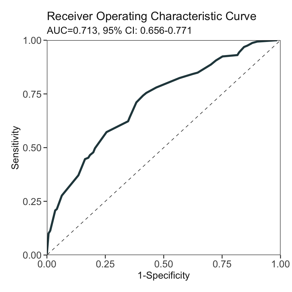
***Performance using AutoScore:
AUC: 0.7133 95% CI: 0.6556-0.7709 (DeLong)
Best score threshold: >= 51
Other performance indicators based on this score threshold:
Sensitivity: 0.7421 95% CI: 0.673-0.805
Specificity: 0.5887 95% CI: 0.5035-0.6667
PPV: 0.6704 95% CI: 0.6236-0.7143
NPV: 0.6696 95% CI: 0.6043-0.735head(pred_score) pred_score Label
1 53 TRUE
2 56 TRUE
3 49 TRUE
4 38 FALSE
5 51 TRUE
6 40 TRUEprint_roc_performance() to generate the performance under different score thresholds (e.g., 90).print_roc_performance(pred_score$Label, pred_score$pred_score, threshold = 90)AUC: 0.7133 95% CI: 0.6556-0.7709 (DeLong)
Score threshold: >= 90
Other performance indicators based on this score threshold:
Sensitivity: 0.0063
Specificity: 1
PPV: 1
NPV: 0.4716conversion_table(). Please refer to our demo for large sample (4.1.6) for detail.In Demo 3, we demonstrate the use of AutoScore on a simulated dataset with missing values in two variables (i.e., Vital_A, Vital_B).
check_data(sample_data_missing)Data type check passed.
WARNING: NA detected in data: ----- Variable name No. missing %missing
Vital_A Vital_A 4000 20
Vital_B Vital_B 12000 60SUGGESTED ACTION:
* Consider imputation and supply AutoScore with complete data. * Alternatively, AutoScore can handle missing values as a separate 'Unknown' category, IF:
- you believe the missingness in your dataset is informative, AND
- missing is prevalent enough that you prefer to preserve them as NA rather than removing or doing imputation, AND
- missing is not too prevalent, which may make results unstable.AutoScore can automatically treat the missingness as a new category named Unknown. The following steps are the same as those in Demo 1 (4.1).
set.seed(4)
out_split <- split_data(data = sample_data_missing, ratio = c(0.7, 0.1, 0.2))
train_set <- out_split$train_set
validation_set <- out_split$validation_set
test_set <- out_split$test_set
ranking <- AutoScore_rank(train_set, method = "rf", ntree = 100)The ranking based on variable importance was shown below for each variable:
Age Lab_H Lab_K Lab_B Vital_E Vital_A Lab_I Lab_A
152.05596 148.65760 145.97057 144.55385 135.95607 120.73739 107.02069 100.41955
Vital_C Lab_M Vital_D Lab_D Lab_J Vital_F Lab_F Lab_E
95.80391 92.82594 88.44859 85.59284 84.37891 82.78763 79.04925 78.03686
Lab_L Lab_C Lab_G Vital_B Vital_G
74.75048 74.11922 58.84757 57.91472 57.76022 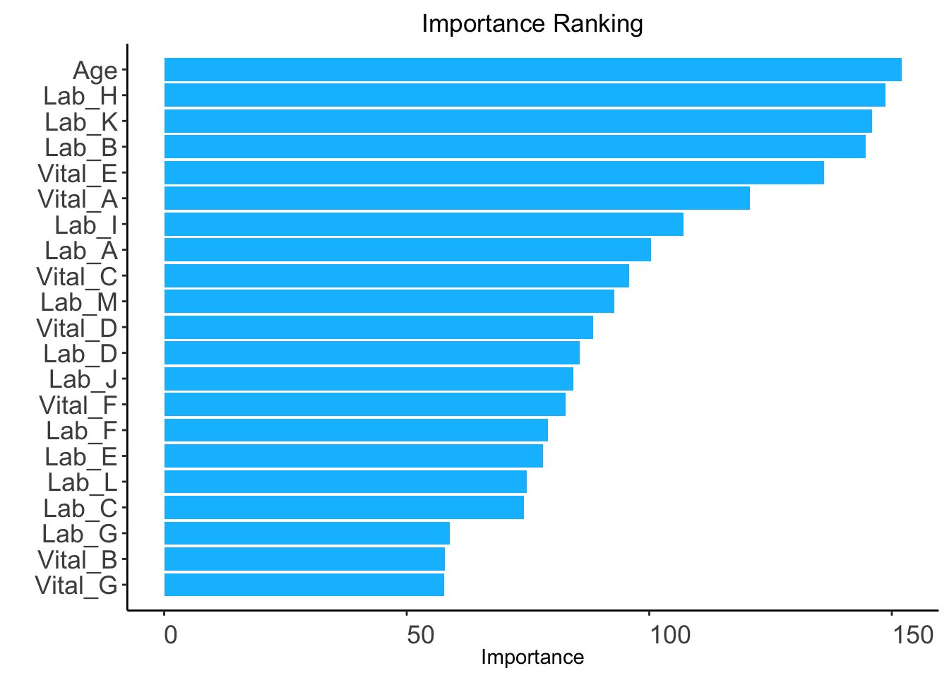
AUC <- AutoScore_parsimony(
  train_set = train_set, validation_set = validation_set,
  rank = ranking, max_score = 100, n_min = 1, n_max = 20,
  categorize = "quantile", quantiles = c(0, 0.05, 0.2, 0.8, 0.95, 1),
  auc_lim_min = 0.5, auc_lim_max = "adaptive"
)
Select 1 Variable(s): Area under the curve: 0.6649
Select 2 Variable(s): Area under the curve: 0.7466
Select 3 Variable(s): Area under the curve: 0.7729
Select 4 Variable(s): Area under the curve: 0.7915
Select 5 Variable(s): Area under the curve: 0.8138
Select 6 Variable(s): Area under the curve: 0.8178
Select 7 Variable(s): Area under the curve: 0.8152
Select 8 Variable(s): Area under the curve: 0.8159
Select 9 Variable(s): Area under the curve: 0.814
Select 10 Variable(s): Area under the curve: 0.8142
Select 11 Variable(s): Area under the curve: 0.8137
Select 12 Variable(s): Area under the curve: 0.8209
Select 13 Variable(s): Area under the curve: 0.823
Select 14 Variable(s): Area under the curve: 0.8264
Select 15 Variable(s): Area under the curve: 0.8244
Select 16 Variable(s): Area under the curve: 0.8213
Select 17 Variable(s): Area under the curve: 0.8232
Select 18 Variable(s): Area under the curve: 0.8223
Select 19 Variable(s): Area under the curve: 0.8159
Select 20 Variable(s): Area under the curve: 0.8243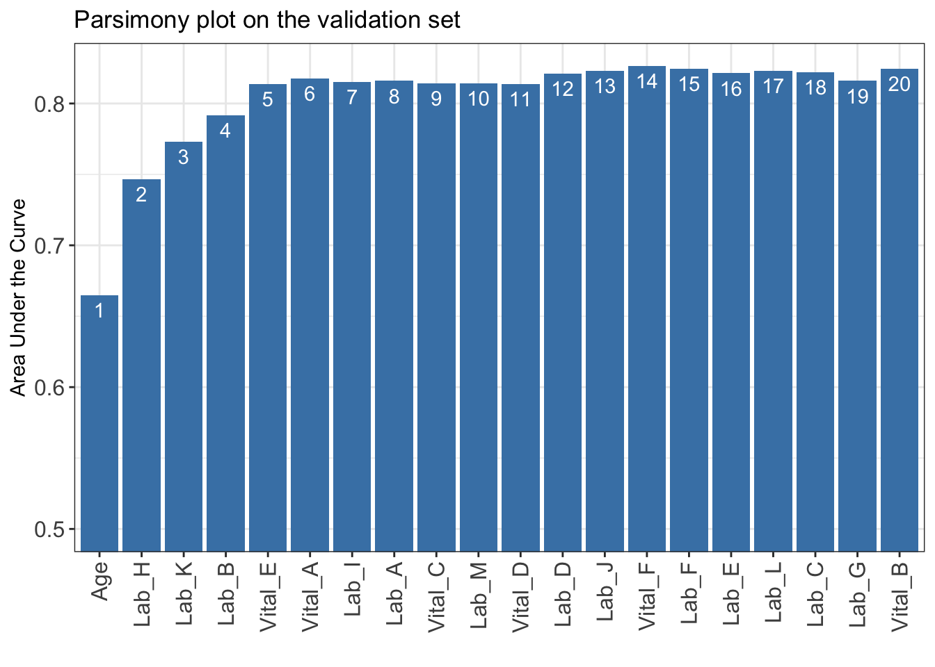
Unknown category indicating the missingness will be displayed in the final scoring table.num_var <- 6
final_variables <- names(ranking[1:num_var])
cut_vec <- AutoScore_weighting(
  train_set = train_set, validation_set = validation_set,
  final_variables = final_variables, max_score = 100,
  categorize = "quantile", quantiles = c(0, 0.05, 0.2, 0.8, 0.95, 1)
)
****Included Variables:
variable_name
1 Age
2 Lab_H
3 Lab_K
4 Lab_B
5 Vital_E
6 Vital_A
****Initial Scores:
======== ========== =====
variable interval point
======== ========== =====
Age <35 0
[35,49) 8
[49,76) 17
[76,89) 22
>=89 26
Lab_H <0.2 0
[0.2,1.1) 4
[1.1,3.1) 9
[3.1,4) 14
>=4 18
Lab_K <8 0
[8,42) 7
[42,58) 11
>=58 14
Lab_B <8.5 0
[8.5,11.2) 4
[11.2,17) 7
[17,19.8) 11
>=19.8 12
Vital_E <12 0
[12,15) 1
[15,22) 8
[22,25) 13
>=25 16
Vital_A <59 1
[59,70) 0
[70,100) 7
[100,112) 12
>=113 13
Unknown 7
======== ========== =====
***Performance (based on validation set):
AUC:  0.8178   95% CI: 0.785-0.8506 (DeLong)
Best score threshold: >= 57
Other performance indicators based on this score threshold:
Sensitivity: 0.8581
Specificity: 0.6054
PPV:         0.1545
NPV:         0.9807
***The cutoffs of each variable generated by the AutoScore are saved in cut_vec. You can decide whether to revise or fine-tune them