6AutoScore for ordinal outcomes (AutoScore-Ordinal)
AutoScore-Ordinal refers to the AutoScore framework for developing point-based scoring models for ordinal outcomes. Similar to the implementation described in Chapter 4 for binary outcomes, AutoScore-Ordinal is implemented by five functions: AutoScore_rank_Ordinal(), AutoScore_parsimony_Ordinal(), AutoScore_weighting_Ordinal(), AutoScore_fine_tuning_Ordinal() and AutoScore_testing_Ordinal().
In this chapter, we demonstrate the use of AutoScore-Ordinal to develop sparse risk scores for an ordinal outcome, adjust parameters to improve interpretability, assess the performance of the final model and map the score to predict risks for new data. To facilitate clinical applications, in the following sections we demonstrate AutoScore application in 3 demos with large and small datasets and with missing information.
Important
Scoring models below are based on simulated data to demonstrate AutoScore usage.
Variable names are intentionally masked to avoid misinterpretation and misuse.
In Demo 1, we demonstrate the use of AutoScore-Ordinal on a dataset with 20,000 observations using split-sample approach (i.e., to randomly divide the full dataset into training, validation and test sets) for model development.
Important
Before proceeding, follow the steps in Chapter 2 to ensure all data requirements are met.
Refer to Chapter 3 for how to generate simple descriptive statistics before building prediction models.
Option 1: Prepare three separate datasets to train, validate, and test models.
Option 2: Use demo codes below to randomly split your dataset into training, validation, and test datasets (70%, 10%, 20%, respectively), possibly stratified by outcome categories (strat_by_label = TRUE) to ensure they are well represented in all three datasets.
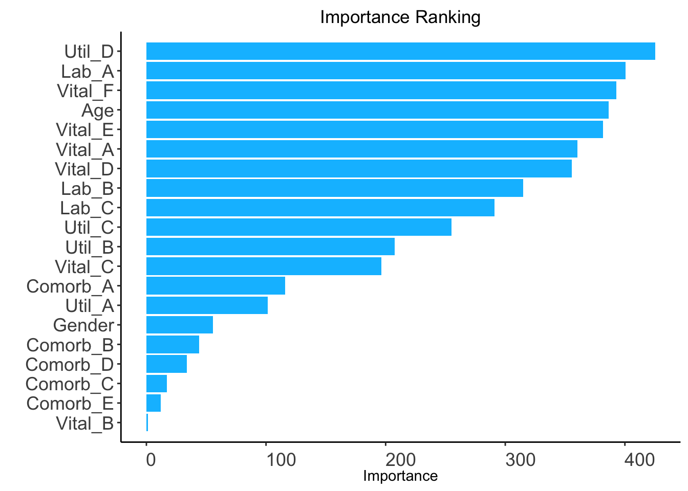
The ranking based on variable importance was shown below for each variable:
   Util_D     Lab_A   Vital_F   Vital_A       Age   Vital_E   Vital_D     Lab_B
413.60631 379.51127 378.30195 372.84319 372.68880 364.51371 339.60643 296.86038
    Lab_C    Util_C    Util_B   Vital_C   Vital_B  Comorb_A    Util_A    Gender
279.47643 244.28653 201.34337 186.47331 168.45639 115.28191  98.78811  51.88705
 Comorb_B  Comorb_D  Comorb_C  Comorb_E
 41.11154  32.31979  17.64803  11.87098
6.1.2 STEP(ii): select model with parsimony plot
AutoScore-Ordinal Modules 2+3+4
n_min: Minimum number of selected variables (Default: 1).
n_max: Maximum number of selected variables (Default: 20).
categorize: Methods for categorizing continuous variables. Options include "quantile" or "kmeans" (Default: "quantile").
quantiles: Predefined quantiles to convert continuous variables to categorical ones. (Default: c(0, 0.05, 0.2, 0.8, 0.95, 1)) Available if categorize = "quantile".
max_cluster: The maximum number of cluster (Default: 5). Available if categorize = "kmeans".
max_score: Maximum total score (Default: 100).
auc_lim_min: Minimum y_axis limit in the parsimony plot (Default: 0.5).
auc_lim_max: Maximum y_axis limit in the parsimony plot (Default: “adaptive”).
link: link function in the ordinal regression, which affects predictive performance. Options include "logit" (for proportional odds model), "cloglog" (for proportional hazard model) and "probit" (Default: "logit").
Important
Use the same link parameter throughout descriptive analysis and model building steps.
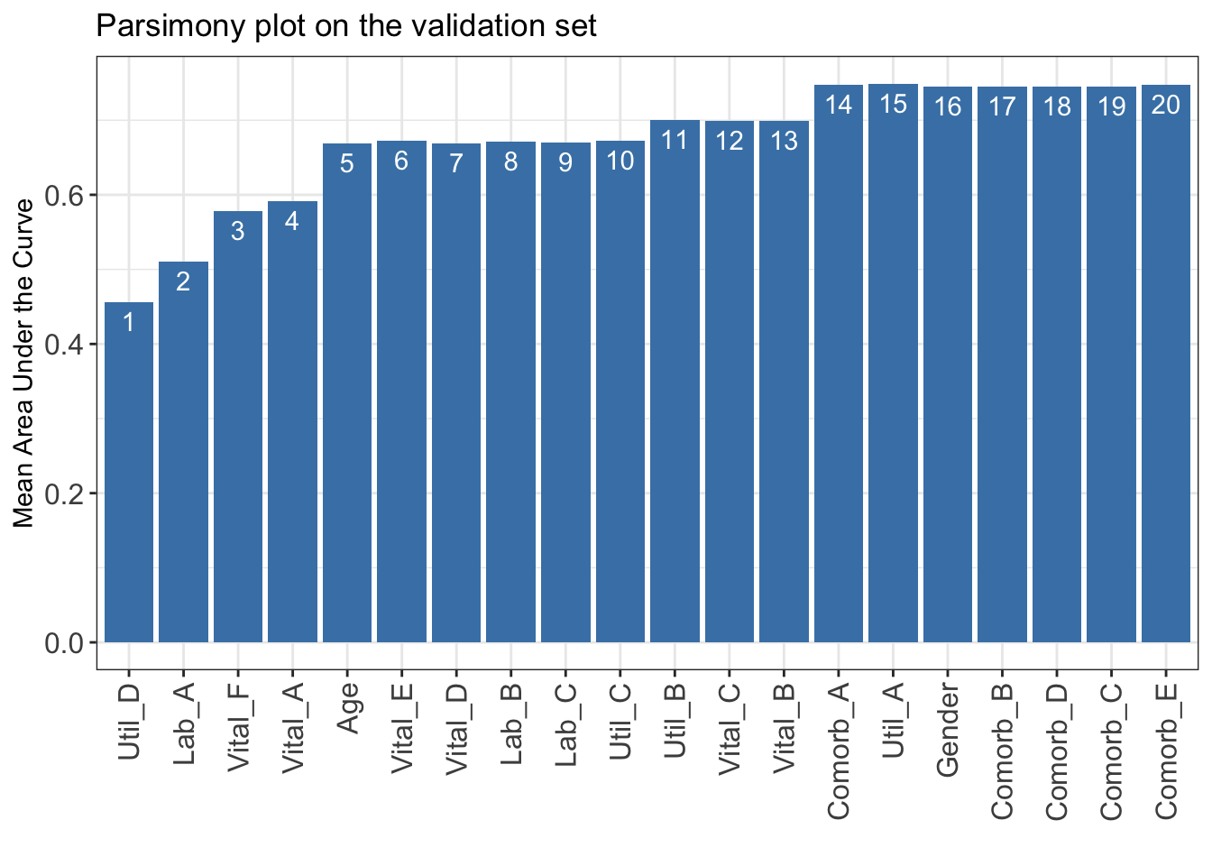
Select 1 variables:  Mean area under the curve: 0.4555607
Select 2 variables:  Mean area under the curve: 0.5110174
Select 3 variables:  Mean area under the curve: 0.5780548
Select 4 variables:  Mean area under the curve: 0.5912554
Select 5 variables:  Mean area under the curve: 0.6685143
Select 6 variables:  Mean area under the curve: 0.672106
Select 7 variables:  Mean area under the curve: 0.6690071
Select 8 variables:  Mean area under the curve: 0.6710102
Select 9 variables:  Mean area under the curve: 0.6706072
Select 10 variables:  Mean area under the curve: 0.6721932
Select 11 variables:  Mean area under the curve: 0.7003498
Select 12 variables:  Mean area under the curve: 0.6995013
Select 13 variables:  Mean area under the curve: 0.6994186
Select 14 variables:  Mean area under the curve: 0.7476355
Select 15 variables:  Mean area under the curve: 0.7489346
Select 16 variables:  Mean area under the curve: 0.7448716
Select 17 variables:  Mean area under the curve: 0.744752
Select 18 variables:  Mean area under the curve: 0.744752
Select 19 variables:  Mean area under the curve: 0.745261
Select 20 variables:  Mean area under the curve: 0.7472124
Note
Users could use mAUC for further analysis or export it to CSV to other software for plotting.
write.csv(data.frame(mAUC), file ="mAUC.csv")
Determine the optimal number of variables (num_var) based on the parsimony plot obtained in STEP(ii).
The final list of variables is the first num_var variables in the ranked list ranking obtained in STEP(i).
Optional: User can adjust the finally included variables final_variables based on the clinical preferences and knowledge.
# Example 1: Top 5 variables are selectednum_var <-5final_variables <-names(ranking[1:num_var])# Example 2: Top 14 variables are selectednum_var <-14final_variables <-names(ranking[1:num_var])# Example 3: Top 5 variables, the 11th and 14th variable are selectedfinal_variables <-names(ranking[c(1:5, 11, 14)])
6.1.3 STEP(iii): generate initial scores with final variables
Re-run AutoScore-Ordinal Modules 2+3
Generate cut_vec with current cutoffs of continuous variables, which can be fine-tuned in STEP(iv).
Performance of resulting scores is evaluated using the mean AUC across dichotomous classifications (mAUC), with 95% CI computed using bootstrap (Default: n_boot = 100 bootstrap samples). Setting n_boot = 1 disables bootstrap and reports mAUC without CI.
Run time increases with larger n_boot value. Code below uses n_boot = 10 for demonstration.
Revise cut_vec with domain knowledge to update the scoring table (AutoScore-Ordinal Module 5).
Re-run AutoScore-Ordinal Modules 2+3 to generate the updated scores.
Users can choose any cutoff values and/or any number of categories, but are suggested to choose numbers close to the automatically determined values.
## For example, we have current cutoffs of continuous variable: Age ## ============== =========== =====## variable interval point## ============== =========== =====## Age <27 0 ## [27,46) 4 ## [46,78) 14 ## [78,87) 18 ## >=87 21
Current cutoffs:c(27, 46, 78, 87). We can fine tune the cutoffs as follows:
# Example 1: rounding to a nice numbercut_vec$Age <-c(25, 45, 75, 85)# Example 2: changing cutoffs according to clinical knowledge or preference cut_vec$Age <-c(25, 50, 75, 85)# Example 3: combining categoriescut_vec$Age <-c(45, 75, 85)
mAUC and 95% bootstrap CI (Default: n_boot = 100 bootstrap samples) are reported after fine-tuning.
Run time increases with larger n_boot value. Code below uses n_boot = 10 for demonstration.
Given the proportion of subjects for each score value (see figure above), select reasonable score breaks (Default: 5, 10, 15, …, 70) to report the average predicted risk within each score interval, which can be used to predict risk for a new subject.
When selecting score breaks, avoid creating score intervals with too few observations.
conversion_table_ordinal(pred_score = pred_score, link = link,score_breaks =seq(from =5, to =70, by =5), digits =4)
Score
Predicted risk, category 1
Predicted risk, category 2
Predicted risk, category 3
[0,5]
0.9742
0.0192
0.0065
(5,10]
0.9617
0.0285
0.0098
(10,15]
0.9454
0.0404
0.0142
(15,20]
0.9226
0.0569
0.0205
(20,25]
0.8914
0.0791
0.0295
(25,30]
0.8497
0.1081
0.0423
(30,35]
0.7956
0.1441
0.0602
(35,40]
0.7284
0.1864
0.0851
(40,45]
0.6489
0.2321
0.1190
(45,50]
0.5602
0.2758
0.1640
(50,55]
0.4675
0.3109
0.2216
(55,60]
0.3769
0.3307
0.2924
(60,65]
0.2942
0.3309
0.3749
(65,70]
0.2231
0.3116
0.4653
(70,100]
0.0840
0.1718
0.7442
Note
Users could use pred_score for further analysis or export it to CSV to other software (e.g., generating the calibration curve).
write.csv(pred_score, file ="pred_score.csv")
6.2 Demo 2: small sample
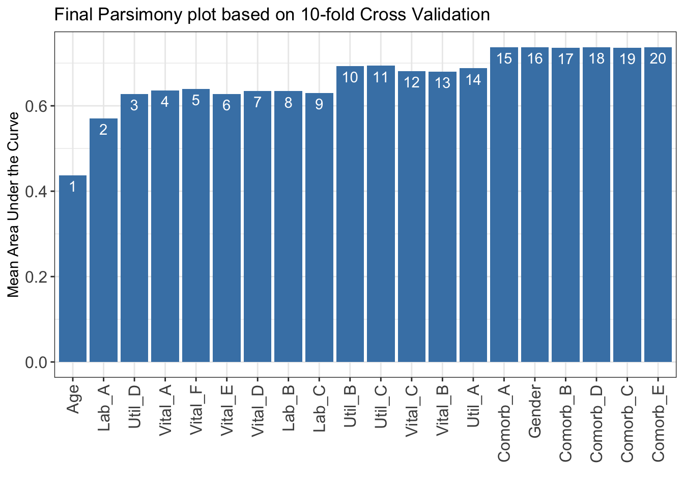
In Demo 2, we demonstrate the use of AutoScore-Ordinal on a smaller dataset where there are no sufficient samples to form a separate training and validation dataset. Thus, the cross validation is employed to generate the parsimony plot.
Load small dataset with 5000 samples
data("sample_data_ordinal_small")
Prepare training and test datasets
Option 1: Prepare two separate datasets to train and test models.
Option 2: Use demo codes below to randomly split your dataset into training and test datasets (70% and 30%, respectively). For cross-validation, train_set is equal to validation_set and the ratio of validation_set should be 0. Then cross-validation will be implemented in the STEP(ii), AutoScore_parsimony_Ordinal().
The ranking based on variable importance was shown below for each variable:
      Age     Lab_A    Util_D   Vital_A   Vital_F   Vital_E   Vital_D     Lab_B
98.791839 98.073161 97.021662 93.282141 92.469166 91.677271 82.051893 72.462999
    Lab_C    Util_B    Util_C   Vital_C   Vital_B    Util_A  Comorb_A    Gender
70.507041 57.778464 57.270171 45.468903 43.633031 26.120379 25.414958 13.405373
 Comorb_B  Comorb_D  Comorb_C  Comorb_E
 9.595971  7.320633  4.477519  2.993603
6.2.2 STEP(ii): select the best model with parsimony plot
AutoScore-Ordinal Modules 2+3+4
nmin: Minimum number of selected variables (Default: 1).
nmax: Maximum number of selected variables (Default: 20).
categorize: Methods for categorizing continuous variables. Options include "quantile" or "kmeans" (Default: "quantile").
quantiles: Predefined quantiles to convert continuous variables to categorical ones. (Default: c(0, 0.05, 0.2, 0.8, 0.95, 1)) Available if categorize = "quantile".
max_cluster: The maximum number of cluster (Default: 5). Available if categorize = "kmeans".
max_score: Maximum total score (Default: 100).
auc_lim_min: Minimum y_axis limit in the parsimony plot (Default: 0.5).
auc_lim_max: Maximum y_axis limit in the parsimony plot (Default: “adaptive”).
cross_validation: TRUE if cross-validation is needed, especially for small datasets.
fold: The number of folds used in cross validation (Default: 10). Available if cross_validation = TRUE.
do_trace: If set to TRUE, all results based on each fold of cross-validation would be printed out and plotted (Default: FALSE). Available if cross_validation = TRUE.
link: link function in the ordinal regression, which affects predictive performance. Options include "logit" (for proportional odds model), "cloglog" (for proportional hazard model) and "probit" (Default: "logit").
Important
Use the same link parameter throughout descriptive analysis and model building steps.
Users could use mAUC for further analysis or export it to CSV to other software for plotting.
write.csv(data.frame(mAUC), file ="mAUC.csv")
Determine the optimal number of variables (num_var) based on the parsimony plot obtained in STEP(ii).
The final list of variables is the first num_var variables in the ranked list ranking obtained in STEP(i).
Optional: User can adjust the finally included variables final_variables based on the clinical preferences and knowledge.
# Example 1: Top 6 variables are selectednum_var <-6final_variables <-names(ranking[1:num_var])# Example 2: Top 14 variables are selectednum_var <-14final_variables <-names(ranking[1:num_var])# Example 3: Top 3 variables, the 10th and 15th variable are selectedfinal_variables <-names(ranking[c(1:3, 10, 15)])
6.2.3 STEP(iii): generate initial scores with final variables
Re-run AutoScore-Ordinal Modules 2+3
Generate cut_vec with current cutoffs of continuous variables, which can be fine-tuned in STEP(iv).
Performance of resulting scores is evaluated using the mean AUC across dichotomous classifications (mAUC), with 95% CI computed using bootstrap (Default: n_boot = 100 bootstrap samples). Setting n_boot = 1 disables bootstrap and reports mAUC without CI.
Revise cut_vec with domain knowledge to update the scoring table (AutoScore-Ordinal Module 5).
Re-run AutoScore-Ordinal Modules 2+3 to generate the updated scores.
Users can choose any cutoff values and/or any number of categories, but are suggested to choose numbers close to the automatically determined values.
## For example, we have current cutoffs of continuous variable: Age ## ============== =========== =====## variable interval point## ============== =========== =====## Age <27 0 ## [27,46) 4 ## [46,78) 14 ## [78,87) 18 ## >=87 21
Current cutoffs:c(27, 46, 78, 87). We can fine tune the cutoffs as follows:
# Example 1: rounding to a nice numbercut_vec$Age <-c(25, 45, 75, 85)# Example 2: changing cutoffs according to clinical knowledge or preference cut_vec$Age <-c(25, 50, 75, 85)# Example 3: combining categoriescut_vec$Age <-c(45, 75, 85)
mAUC and 95% bootstrap CI (Default: n_boot = 100 bootstrap samples) are reported after fine-tuning.
Run time increases with larger n_boot value. Code below uses n_boot = 10 for demonstration.
Users can also map score to risk using plot_predicted_risk() and conversion_table_ordinal(). Please refer to our demo for large sample (6.1.6) for detail.
6.3 Demo 3: data with missing values
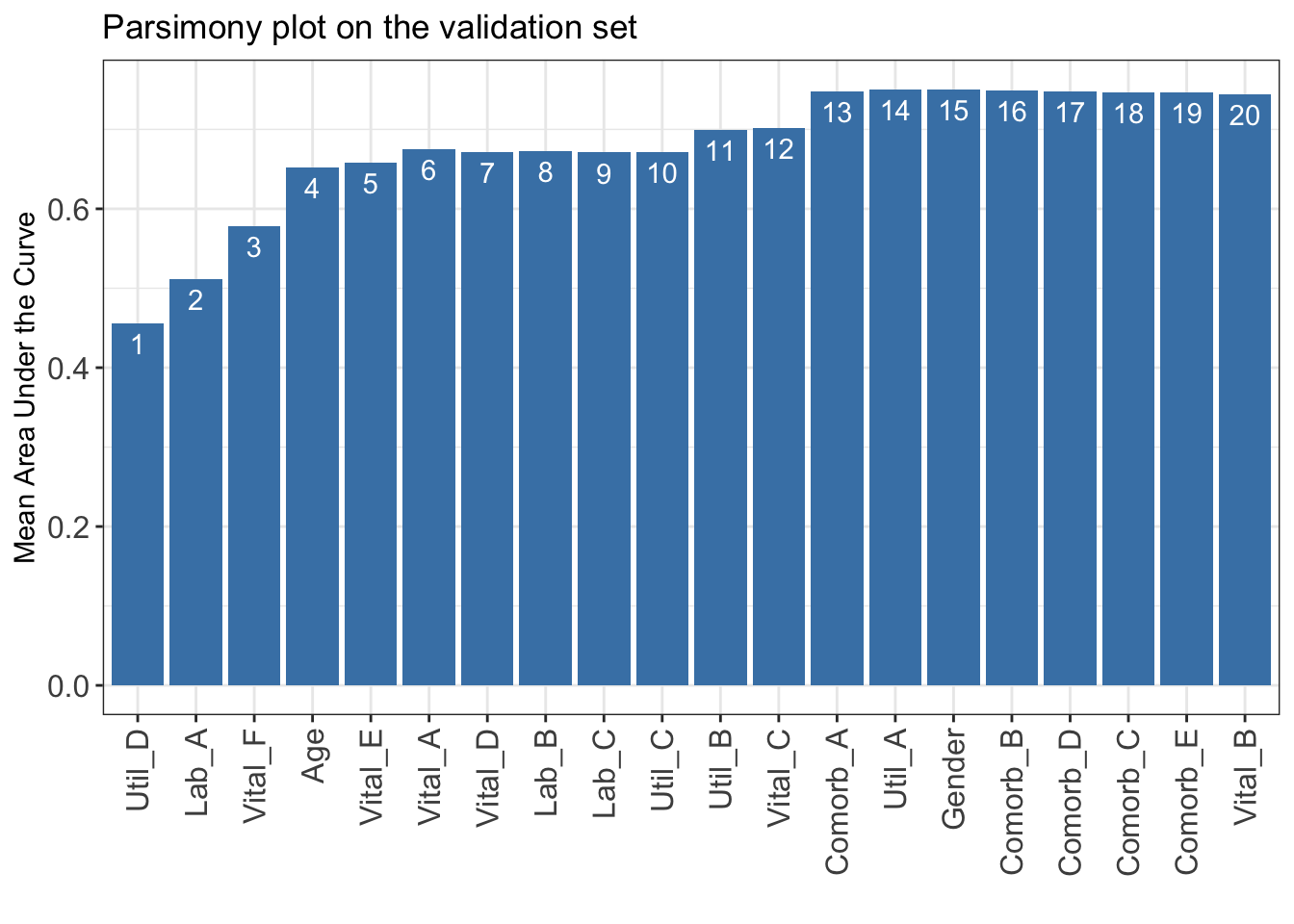
In Demo 3, we demonstrate AutoScore-Ordinal for application to data with missing values in two variables (i.e., Vital_A, Vital_B).
SUGGESTED ACTION:
 * Consider imputation and supply AutoScore with complete data.
 * Alternatively, AutoScore can handle missing values as a separate 'Unknown' category, IF:
    - you believe the missingness in your dataset is informative, AND
    - missing is prevalent enough that you prefer to preserve them as NA rather than removing or doing imputation, AND
    - missing is not too prevalent, which may make results unstable.
AutoScore can automatically treat the missingness as a new category named Unknown. The following steps are the same as those in Demo 1 (6.1).
Important
High missing rate may cause the variable ranking less reliable, and thus, caution is needed for variable selection using parsimony plot.
Select 1 variables:  Mean area under the curve: 0.4555607
Select 2 variables:  Mean area under the curve: 0.5110174
Select 3 variables:  Mean area under the curve: 0.5780548
Select 4 variables:  Mean area under the curve: 0.6524352
Select 5 variables:  Mean area under the curve: 0.6579466
Select 6 variables:  Mean area under the curve: 0.675316
Select 7 variables:  Mean area under the curve: 0.6714668
Select 8 variables:  Mean area under the curve: 0.6731644
Select 9 variables:  Mean area under the curve: 0.6709335
Select 10 variables:  Mean area under the curve: 0.671352
Select 11 variables:  Mean area under the curve: 0.6993675
Select 12 variables:  Mean area under the curve: 0.7013214
Select 13 variables:  Mean area under the curve: 0.7473641
Select 14 variables:  Mean area under the curve: 0.7504558
Select 15 variables:  Mean area under the curve: 0.7501569
Select 16 variables:  Mean area under the curve: 0.7495503
Select 17 variables:  Mean area under the curve: 0.7478535
Select 18 variables:  Mean area under the curve: 0.7470084
Select 19 variables:  Mean area under the curve: 0.7468875
Select 20 variables:  Mean area under the curve: 0.7444887
Note
The Unknown category indicating the missingness will be displayed in the final scoring table.