from ShapleyVIC import df_compas

compas = df_compas.load_data()
# See data description using the following command:
# help(df_compas.load_data)
compas.loc[:5]2 ShapleyVIC for Variable Importance Assessment
ShapleyVIC is model agnostic, and its benefits of has been demonstrated in empirical experiments in applications for multiple domains. This tutorial illustrates ShapleyVIC implementation using the Python library and R package, in a study with a binary outcome that predicts 2-year recidivism using a logistic regression of 6 binary variables. Chapter 5 and Chapter 6 provides reproducible examples for ShapleyVIC analysis of ordinal and continuous outcomes, respectively.
Cite the following papers for ShapleyVIC:
- Ning Y, Ong ME, Chakraborty B, Goldstein BA, Ting DS, Vaughan R, Liu N. Shapley variable importance cloud for interpretable machine learning. Patterns 2022; 3: 100452.
2.1 [Python] ShapleyVIC calculation
This part of the ShapleyVIC workflow is implemented in Python.
In this part of the workflow, we load and prepare data, train optimal logistic regression model, generate nearly optimal models, and compute Shapley-based variable importance for each model.
2.1.1 Load data
- Read data from CSV or Excel files.
- For this demo, use the integrated data in the library that contains 7214 samples analyzed in Experiment 1 (i.e., the recidivism prediction study) of the paper.
| y | age | race | prior | gender | juvenilecrime | currentcharge | train_test |
|---|---|---|---|---|---|---|---|
| 0 | 0 | 0 | 1 | 1 | 1 | 0 | train |
| 1 | 0 | 1 | 1 | 1 | 1 | 0 | train |
| 1 | 0 | 1 | 0 | 1 | 0 | 0 | train |
| 0 | 0 | 1 | 0 | 1 | 0 | 0 | train |
| 0 | 0 | 0 | 0 | 1 | 1 | 0 | train |
| 0 | 0 | 0 | 1 | 1 | 1 | 1 | train |
- y: 2-year recidivism (the binary outcome, 1=event and 0=non-event).
- age, race, prior, gender, juvenilecrime, currentcharge: binary predictors.
- train_test: training/explanation set membership indicator (
"train"for training and"test"for explanation). Not to include in models.
2.1.2 Prepare training and explanation sets
- When there is sufficient data, users can split the full dataset into a training set to train optimal and nearly optimal models, and an explanation set to compute ShapleyVIC values.
- Otherwise, users may use the full dataset to train models and compute ShapleyVIC values.
Important
- As detailed in Chapter 1, check for and handle data issues before applying ShapleyVIC.
- This demo will show impact of data sparsity on ShapleyVIC results.
In the experiment, we used 10% of the full dataset as explanation set. See Chapter 1 for general suggestions on the size of explanation set.
dat_train = compas.loc[compas['train_test']=='train']
# Drop the indicator column after using it to split data:
dat_train = dat_train.drop(columns=['train_test'])
dat_train.reset_index(drop=True, inplace=True)

dat_expl = compas.loc[compas['train_test']=='test']
dat_expl = dat_expl.drop(columns=['train_test'])
dat_expl.reset_index(drop=True, inplace=True)
# Drop the column 'train_test' that indicates set membership in example data:
compas = compas.drop(columns=['train_test'])
# Generate row indices for training and explanation sets:
from sklearn.model_selection import train_test_split
i_train, i_expl = train_test_split(list(range(compas.shape[0])),
test_size=int(0.1 * compas.shape[0]), random_state=0)
dat_train = compas.iloc[i_train, :]
dat_train.reset_index(drop=True, inplace=True)
dat_expl = compas.iloc[i_expl, :]
dat_expl.reset_index(drop=True, inplace=True)2.1.3 Train optimal model
- Specify training data to initialize the model object and train the optimal model.
x,y: predictors (as a data frame) and outcome from the training set.outcome_type: type of the outcome. Default is “binary” that is most common in clinical applications.x_names_cat: names of categorical predictors. Optional for binary predictors encoded as 0/1.output_dir: the directory to save key outputs to. Will be used as input in the subsequent R workflow.save_data: whether to savexandytooutput_dir(default is to save). If not,xandymust be supplied separately in subsequent R analysis.
In this step, users also need to configure the criterion for defining nearly optimal models (see following sections for detail).
- Default is
criterion="loss"that applies to all outcome types, where nearly optimal models exceed minimum loss by no more thanepsilon(default is 0.05, i.e., 5%). criterion="auc"orcriterion="prauc"is also supported for binary outcomes (but not other outcome types), where nearly optimal models have AUC or PRAUC within the 95% of that for the optimal model.
Define nearly optimal based on loss, and epsilon = 0.05 (the default) for the range of permissible loss.
Default option is to save input data x and y, so that they are not needed as input in the subsequent R workflow.
# Specify the name of outcome, which is 'y' in this example:
y_name = 'y'
from ShapleyVIC import model
model_object = model.models(
    x=dat_train.drop(columns=[y_name]), y=dat_train[y_name],
    outcome_type="binary",
    x_names_cat=['age','race','prior','gender','juvenilecrime','currentcharge'],
    output_dir="compas_output"
)
# To display the optimal logistic regression trained:
model_object.model_optim.summary().tables[1]
Define nearly optimal based on AUC, in this case epsilon is not used. This specification does not affect the optimal model.
Users are advised to allocate different output folders when different criterion is selected to avoid confusion. In this example, results are saved to output folder compas_auc_output.
# Specify the name of outcome, which is 'y' in this example:
y_name = 'y'
from ShapleyVIC import model
model_object_auc = model.models(
    x=dat_train.drop(columns=[y_name]), y=dat_train[y_name],
    outcome_type="binary", criterion="auc",
    x_names_cat=['age','race','prior','gender','juvenilecrime','currentcharge'],
    output_dir="compas_auc_output"
)
# To display the optimal logistic regression trained:
model_object_auc.model_optim.summary().tables[1]
Define nearly optimal based on PRAUC, in this case epsilon is not used. This specification does not affect the optimal model.
Users are advised to allocate different output folders when different criterion is selected to avoid confusion. In this example, results are saved to output folder compas_prauc_output.
# Specify the name of outcome, which is 'y' in this example:
y_name = 'y'
from ShapleyVIC import model
model_object_prauc = model.models(
    x=dat_train.drop(columns=[y_name]), y=dat_train[y_name],
    outcome_type="binary", criterion="prauc",
    x_names_cat=['age','race','prior','gender','juvenilecrime','currentcharge'],
    output_dir="compas_prauc_output"
)
# To display the optimal logistic regression trained:
model_object_prauc.model_optim.summary().tables[1]
Specify save_data=False to avoid saving x and y to output folder. See Chapter 3 for another example.
# Specify the name of outcome, which is 'y' in this example:
y_name = 'y'
from ShapleyVIC import model
model_object = model.models(
    x=dat_train.drop(columns=[y_name]), y=dat_train[y_name],
    outcome_type="binary",
    x_names_cat=['age','race','prior','gender','juvenilecrime','currentcharge'],
    output_dir="compas_output", save_data=False
)
# To display the optimal logistic regression trained:
model_object.model_optim.summary().tables[1]| coef | std err | z | P | [0.025 | 0.975] | |
|---|---|---|---|---|---|---|
| const | 0.4455 | 0.107 | 4.160 | 0.000 | 0.236 | 0.655 |
| age | 1.5001 | 0.187 | 8.011 | 0.000 | 1.133 | 1.867 |
| race | 0.4164 | 0.053 | 7.858 | 0.000 | 0.313 | 0.520 |
| prior | -0.8543 | 0.061 | -13.984 | 0.000 | -0.974 | -0.735 |
| gender | 0.3835 | 0.068 | 5.651 | 0.000 | 0.251 | 0.517 |
| juvenilecrime | -0.8646 | 0.084 | -10.238 | 0.000 | -1.030 | -0.699 |
| currentcharge | -0.2544 | 0.056 | -4.562 | 0.000 | -0.364 | -0.145 |
2.1.4 Generate nearly optimal models
As mentioned above, by default (i.e., criterion="loss", epsilon = 0.05) nearly optimal logistic regression models are defined as models with logistic loss less than \((1+\varepsilon)\) times the minimum loss (i.e., logistic loss of the optimal model). Default value for \(\varepsilon\) is 5%.
When criterion="auc" or criterion="prauc" is specified, nearly optimal logistic regression models are defined as models with AUC (or PRAUC) within the 95% CI of that of the optimal logistic regression model.
The criterion (and epsilon) specified when initializing the model object is used to configure and sample nearly optimal models in the following steps.
u1andu2are key hyper-parameters for generating nearly optimal models, which control the sampling range of initial models to fully explore the model space.- Use the following command to generate a set of reasonable values for
u1andu2(usingm=200initial models), such that approximately 70%-80% of initial models are eligible.- The same command applies for all
criterionbut output varies.
- The same command applies for all
u1, u2 = model_object.init_hyper_params(m=200)
(u1, u2)
Nearly optimal defined based on loss with epsilon=0.05.
(0.5, 80.3125)u1, u2 = model_object_auc.init_hyper_params(m=200)
(u1, u2)Nearly optimal defined based on auc.
(0.5, 38.125)u1, u2 = model_object_prauc.init_hyper_params(m=200)
(u1, u2)Nearly optimal defined based on prauc.
(0.5, 32.5)- Use the following command to generate a final set of nearly optimal models (e.g.,
n_final=250) from 500 initial samples (m=500).- The same command applies for all
criterionbut outputs vary.
- The same command applies for all
model_object.draw_models(u1=u1, u2=u2, m=500, n_final=250, random_state=1234)
model_object.models_plot

model_object.models_near_optim.iloc[:5]| const | age_1 | race_1 | prior_1 | gender_1 | juvenilecrime_1 | currentcharge_1 | perf_metric |
|---|---|---|---|---|---|---|---|
| -0.2307 | 3.1195 | 0.5047 | -1.1409 | 0.2644 | -0.1170 | 0.2664 | 1.0280 |
| 0.5503 | 0.7759 | 0.8971 | -1.1164 | -0.3083 | -0.6398 | -0.1481 | 1.0285 |
| 0.1068 | 0.8697 | -0.0176 | -0.6963 | 0.6987 | -0.5041 | -0.1812 | 1.0187 |
| 0.9715 | 0.8669 | -0.1101 | -1.0772 | 0.6450 | -1.3590 | -0.3310 | 1.0212 |
| -1.0476 | 2.0026 | 0.6911 | -0.3203 | 1.4661 | -0.6633 | -0.0397 | 1.0438 |
| 0.4006 | 1.6629 | 0.1719 | -0.5450 | 0.3218 | -0.9498 | 0.6260 | 1.0445 |
model_object_auc.draw_models(u1=u1, u2=u2, m=500, n_final=250, random_state=1234)
model_object_auc.models_plot

model_object_auc.models_near_optim.iloc[:5]| const | age_1 | race_1 | prior_1 | gender_1 | juvenilecrime_1 | currentcharge_1 | perf_metric |
|---|---|---|---|---|---|---|---|
| 0.1989 | 2.5653 | 0.5665 | -1.6820 | 0.7333 | -0.4778 | -0.5296 | 0.6742 |
| 0.5184 | 0.9964 | 0.7507 | -1.0366 | -0.0977 | -0.7082 | -0.1805 | 0.6671 |
| 0.8325 | 1.7529 | 0.5860 | -1.0563 | 0.0572 | -0.8658 | -0.2591 | 0.6785 |
| 0.2104 | 1.0626 | 0.1152 | -0.7446 | 0.6022 | -0.6144 | -0.2036 | 0.6758 |
| 0.8113 | 1.0597 | 0.0502 | -1.0093 | 0.5654 | -1.2084 | -0.3077 | 0.6751 |
| 0.4500 | 1.7156 | 0.4195 | -0.9999 | 0.4521 | -0.7532 | -0.5512 | 0.6765 |
model_object_prauc.draw_models(u1=u1, u2=u2, m=500, n_final=250, random_state=1234)
model_object_prauc.models_plot

model_object_prauc.models_near_optim.iloc[:5]| const | age_1 | race_1 | prior_1 | gender_1 | juvenilecrime_1 | currentcharge_1 | perf_metric |
|---|---|---|---|---|---|---|---|
| 0.2178 | 2.4837 | 0.5550 | -1.6186 | 0.7065 | -0.5075 | -0.5085 | 0.6557 |
| 0.5161 | 1.4747 | 0.5260 | -0.7212 | 0.3116 | -0.9734 | -0.3726 | 0.6636 |
| 0.7843 | 1.0923 | 0.0772 | -0.9979 | 0.5519 | -1.1830 | -0.3038 | 0.6605 |
| 0.4497 | 1.6994 | 0.4193 | -0.9889 | 0.4469 | -0.7616 | -0.5288 | 0.6631 |
| -0.3412 | 0.7137 | 0.3837 | -0.9295 | 1.2320 | -0.6347 | -0.2812 | 0.6622 |
| -0.5807 | 0.5378 | 0.9135 | -0.9719 | 0.6827 | -0.4119 | -0.4054 | 0.6583 |
2.1.5 Assess variable importance
This step assesses variable importance for each nearly optimal model generated in the previous step using the SAGE method, and write the results to the output folder for further processing in the subsequent R workflow. Parallel processing is used to reduce run time.
model_object: the model object created above.x_expl,y_expl: predictors (as a data frame) and outcome from the explanation set.n_cores: number of CPU cores to use in parallel processing.- For a computer with
ncores, do not use more thann-1cores.
- For a computer with
threshold: threshold parameter used in SAGE algorithm for convergence criterion. A reasonable value is 0.05 (default).- Smaller
thresholdvalue may improve accuracy of uncertainty measure but notably increases run time.
- Smaller
- The same command applies for all
criterion.
from ShapleyVIC import compute
m_svic = compute.compute_shapley_vic(
    model_obj=model_object,
    x_expl=dat_expl.drop(columns=[y_name]), y_expl=dat_expl[y_name],
    n_cores=7, # running on a MacBook Air with 8 cores
    threshold=0.05
)
from ShapleyVIC import compute
m_svic = compute.compute_shapley_vic(
model_obj=model_object_auc,
x_expl=dat_expl.drop(columns=[y_name]), y_expl=dat_expl[y_name],
n_cores=7, # running on a MacBook Air with 8 cores
threshold=0.05
)from ShapleyVIC import compute
m_svic = compute.compute_shapley_vic(
model_obj=model_object_prauc,
x_expl=dat_expl.drop(columns=[y_name]), y_expl=dat_expl[y_name],
n_cores=7, # running on a MacBook Air with 8 cores
threshold=0.05
)
Note
- Use built-in software (e.g., Activity Monitor/Task Manager) to monitor CPU and Memory usage. Avoid taking up 100% CPU, which can slow down computation.
- This step can be time consuming with larger number of variables and/or larger explanation data.
- For users’ reference, the commands above took approximately 10-20 minutes on a 2022 MacBook Air (Apple M2 chip with 8‑core CPU, 8-core GPU; 16GB unified memory; 256GB SSD storage).
2.2 [R] ShapleyVIC summary and visualizations
This part of the ShapleyVIC workflow is implemented in R.
This part of the workflow works on output from Python (all saved in output_dir), pooling information across models to compute (and visualize) overall variable importance and derive ensemble variable rankings.
2.2.1 Compute overall importance
As detailed in the paper, raw Shapley-based variable importance needs to be adjusted based on variable colinearity to derive final ShapleyVIC values.
output_dir: output folder generated from the Python workflow.outcome_type: type of outcome, as specified in the Python workflow.criterion: criterion to define nearly optimal models, as used in the Python workflow.- Loss criterion is assumed by default.
xandy: training data specified in the Python workflow, required ifsave_data=Falsewas specified when setting upmodel.models(...)in Python.x_names_cat: names of categorical variables, as specified in the Python workflow. Used when assessing variable colinearity from the training set. Optional for binary variables coded as 0/1.x_names_display: variable names to use in summary statistics and visualizations. If not provided, column names in the training set will be used.
library(ShapleyVIC)
model_object <- compile_shapley_vic(
  output_dir = "compas_output", outcome_type = "binary",
  x_names_cat = c('age','race','prior','gender','juvenilecrime','currentcharge'),
  x_names = c("Age", "Race", "Prior criminal history", "Gender",
              "Juvenile criminal history", "Current charge")
)
Compiling results for binary outcome using loss criterion to define neaerly optimal models.library(ShapleyVIC)
model_object_auc <- compile_shapley_vic(
output_dir = "compas_auc_output", outcome_type = "binary", criterion = "auc",
x_names_cat = c('age','race','prior','gender','juvenilecrime','currentcharge'),
x_names = c("Age", "Race", "Prior criminal history", "Gender",
"Juvenile criminal history", "Current charge")
)Compiling results for binary outcome using auc criterion to define neaerly optimal models.library(ShapleyVIC)
model_object_prauc <- compile_shapley_vic(
output_dir = "compas_prauc_output", outcome_type = "binary", criterion = "prauc",
x_names_cat = c('age','race','prior','gender','juvenilecrime','currentcharge'),
x_names = c("Age", "Race", "Prior criminal history", "Gender",
"Juvenile criminal history", "Current charge")
)Compiling results for binary outcome using prauc criterion to define neaerly optimal models.When training data was not saved in the Python workflow, they must be supplied as input (x and y) in this step. See Chapter 3 for another example.
# Prepare training data the same way as in Python workflow:
library(ShapleyVIC)
library(dplyr)
data("df_compas")
# Use the `train_test` indicator to filter out training data used in Python workflow:
df_train <- df_compas %>% filter(train_test == "train") %>%
  select(-train_test) %>% as.data.frame()
y_name <- "y"
x_names <- setdiff(names(df_train), y_name)
# Supply x and y when compiling results from Python workflow:
model_object <- compile_shapley_vic(
  output_dir = "compas_output", outcome_type = "binary",
  x = df_train[, x_names], y = df_train[, y_name],
  x_names_cat = c('age','race','prior','gender','juvenilecrime','currentcharge'),
  x_names = c("Age", "Race", "Prior criminal history", "Gender",
              "Juvenile criminal history", "Current charge")
)
2.2.2 Visualize overall variable importance
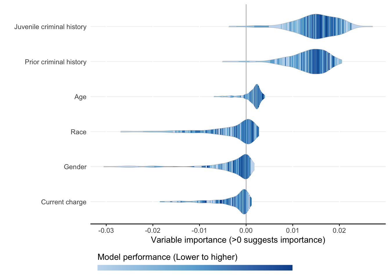
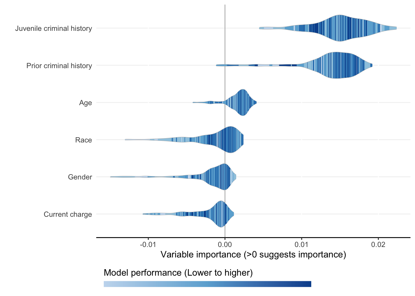
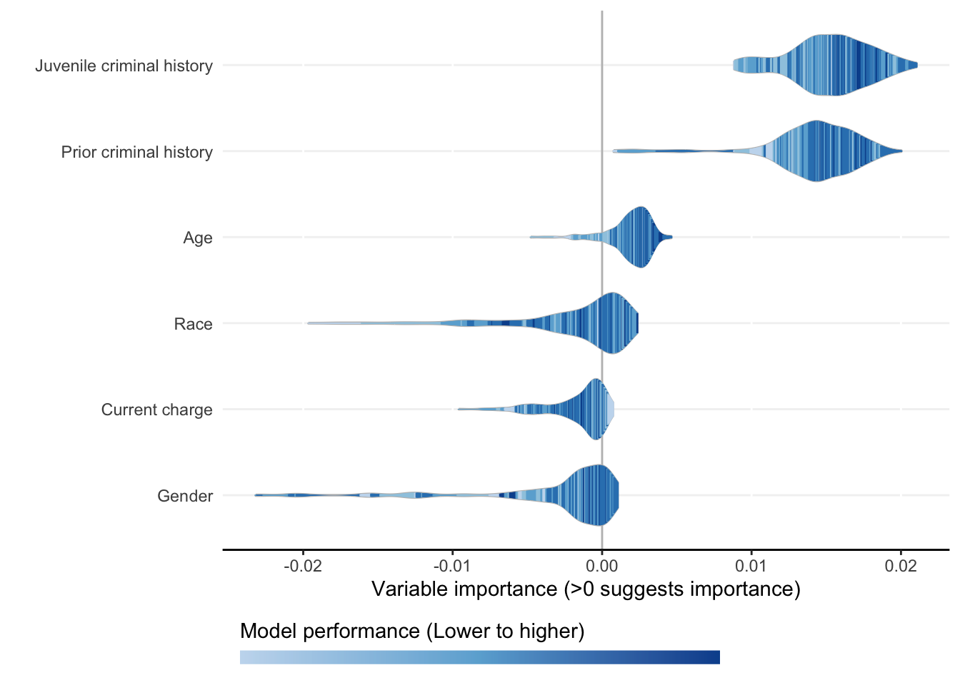
Each ShapleyVIC value (shapley_vic_val) is reported with a standard deviation (sage_sd). We pool information across models to compute overall variable importance and uncertainty interval, visualized using bar plot. The relationship between variable importance and model performance is visualized using violin plot.
- The same command applies for all
criterionand generates similar results. - For clarity, in the bar plot variables with significant overall importance are indicated by blue color and “*” next to variable names.
model_plots <- plot(model_object)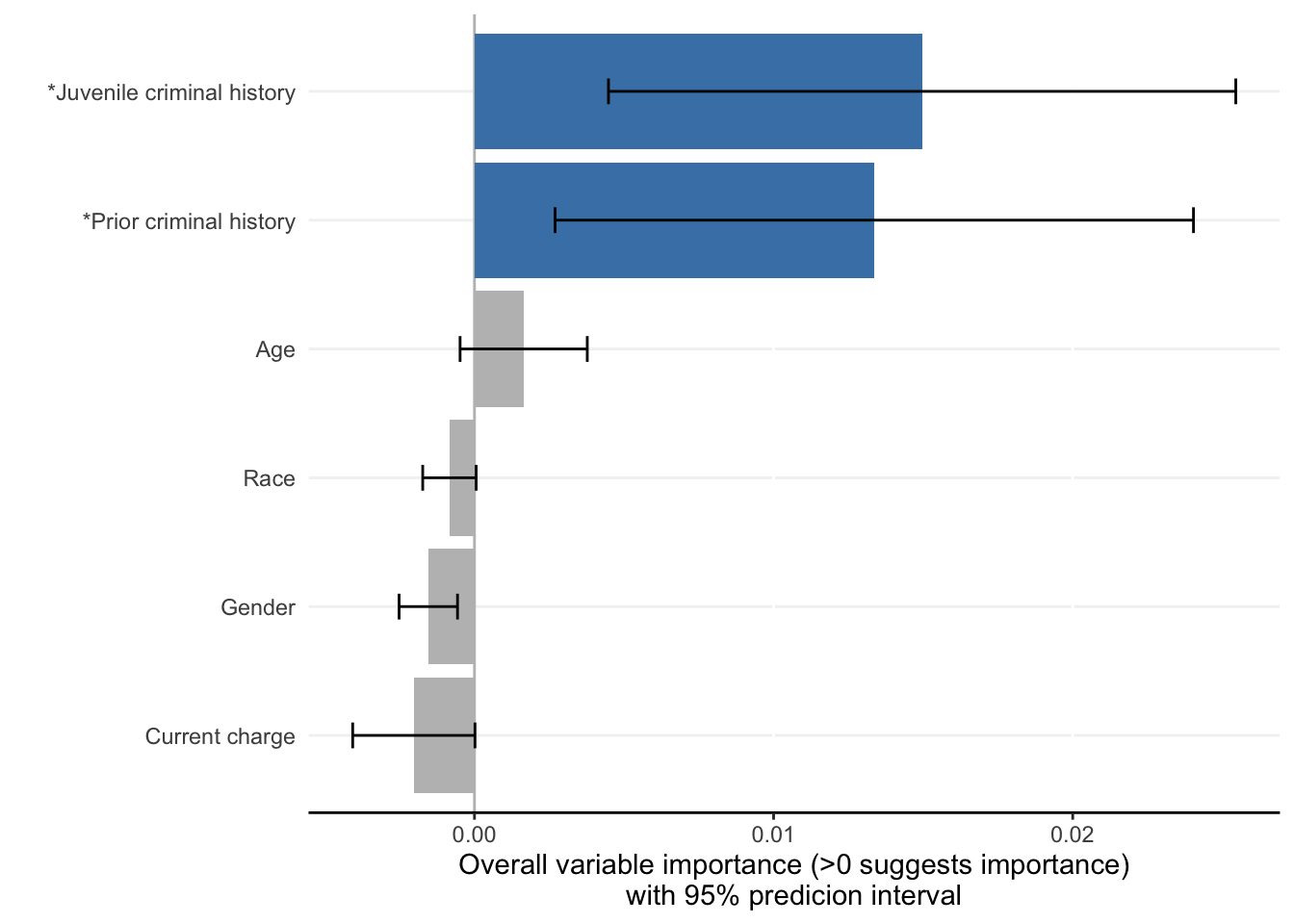
model_auc_plots <- plot(model_object_auc)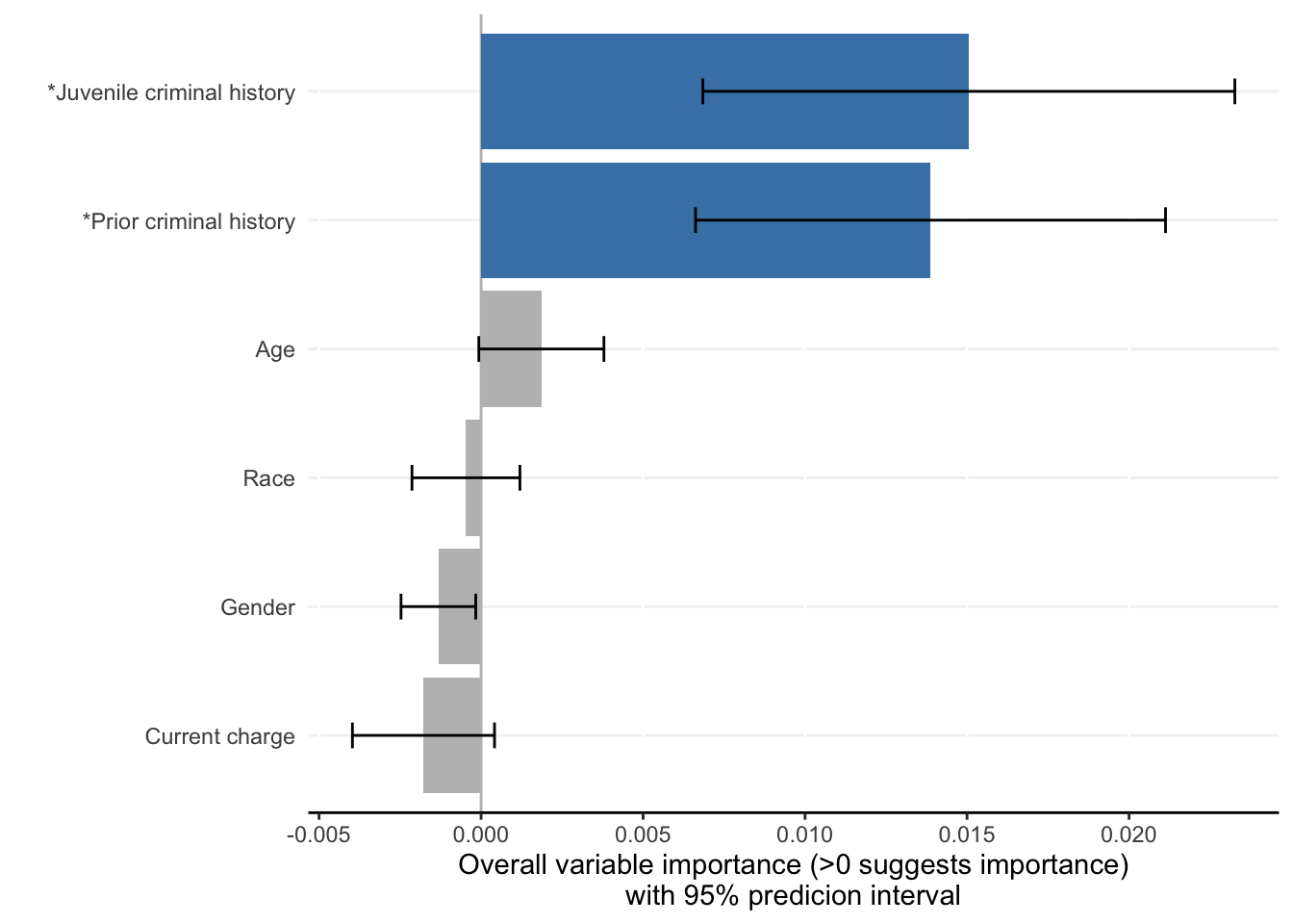
model_prauc_plots <- plot(model_object_prauc)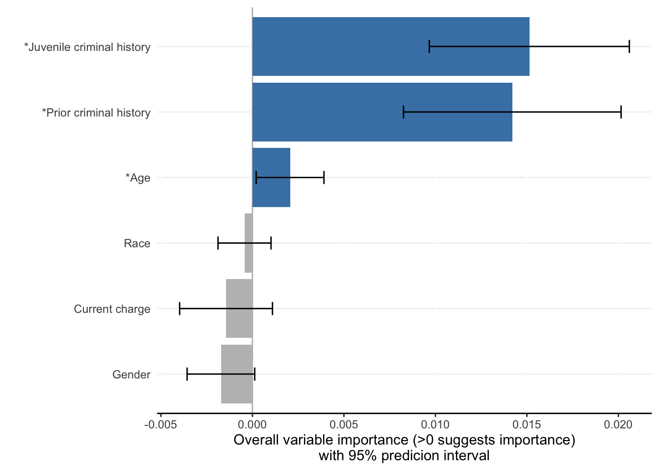
Note
- Plots above reproduce key findings reported in the paper: race had non-significant overall importance, and prior criminal history and juvenile criminal history had higher overall importance than other variables.
- Overall importance of age now becomes non-significant when loss or AUC crterion were used, showing that data sparsity (only 20 [2.8%] of 721 subjects had age=1 in explanation data) leads to less stable results.
The bar plot can be further edited using ggplot functions, e.g., edit text font size using theme() or add plot title using labs():
library(ggplot2)
model_plots$bar + theme(text = element_text(size = 14)) + labs(title = "Bar plot")
To apply similar formatting to the violin plot, use the following function:
library(ggplot2)
plot_violin(x = model_object, title = "Violin plot",
            plot_theme = theme(text = element_text(size = 14)))
2.2.3 Ensemble variable ranking
ShapleyVIC values can also be used to rank variables by their importance to each model. The bar plot of ranks may help identify models with increased reliance on specific variable of interest for further investigation.
The same command applies for all criterion. The example below illustrates for the model object using loss criterion.
val_ranks <- rank_variables(model_object)
head(val_ranks, 6)
model_id Variable rank
1 0 Age 5
2 0 Race 3
3 0 Prior criminal history 1
4 0 Gender 3
5 0 Juvenile criminal history 2
6 0 Current charge 5library(ggplot2)
ggplot(val_ranks, aes(x = rank, group = Variable)) +
geom_bar() +
facet_wrap(~ Variable, nrow = 2) +
theme_bw() +
labs(x = "Ranking", y = "",
title = "ShapleyVIC: Variable ranking among 250 models")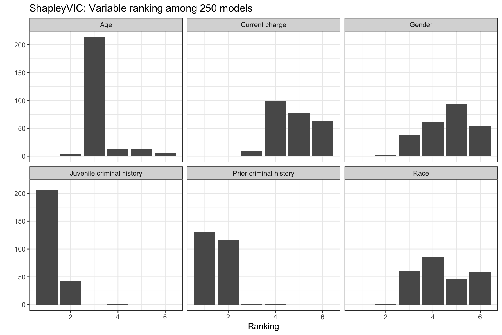
The ensemble ranking averages the ranks across models, and can be used to guide downstream model building, e.g., using AutoScore. See the next chapter for detailed demonstration.
rank_variables(model_object, summarise = TRUE) Variable mean_rank
1 Juvenile criminal history 1.196
2 Prior criminal history 1.492# To return variable ranking as named vector for convenient integration with
# AutoScore:
rank_variables(model_object, summarise = TRUE, as_vector = TRUE)Juvenile criminal history Prior criminal history
1.196 1.492