As introduced in the ShapleyVIC paper, this method can be applied to regression models beyond the logistic regression. This chapter provides a reproducible example to demonstrate its application for continuous outcomes using a simulated dataset from the AutoScore package, which is described in detail in the AutoScore Guidebook.
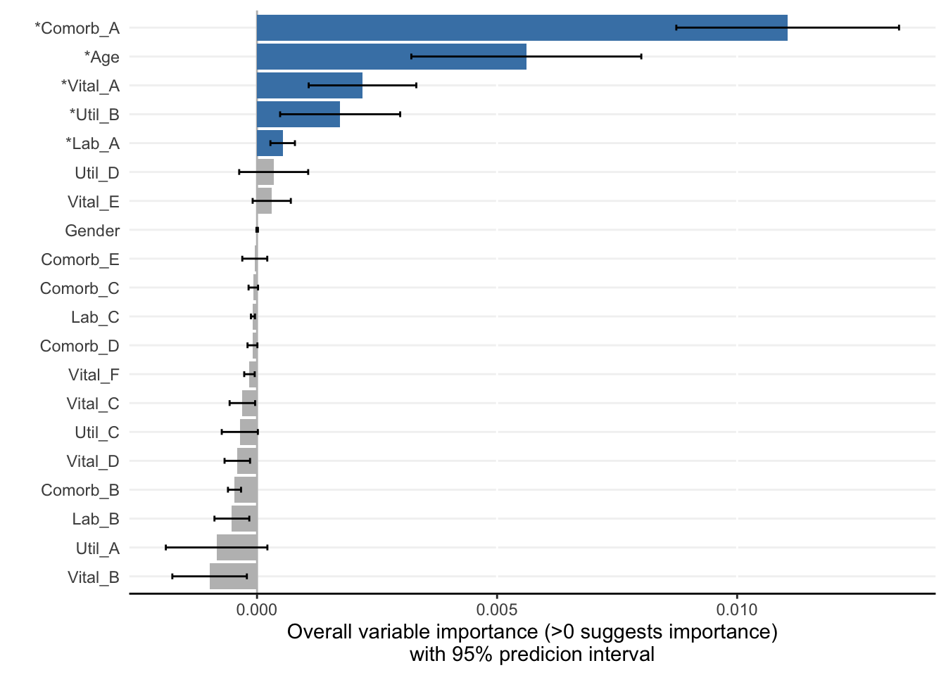
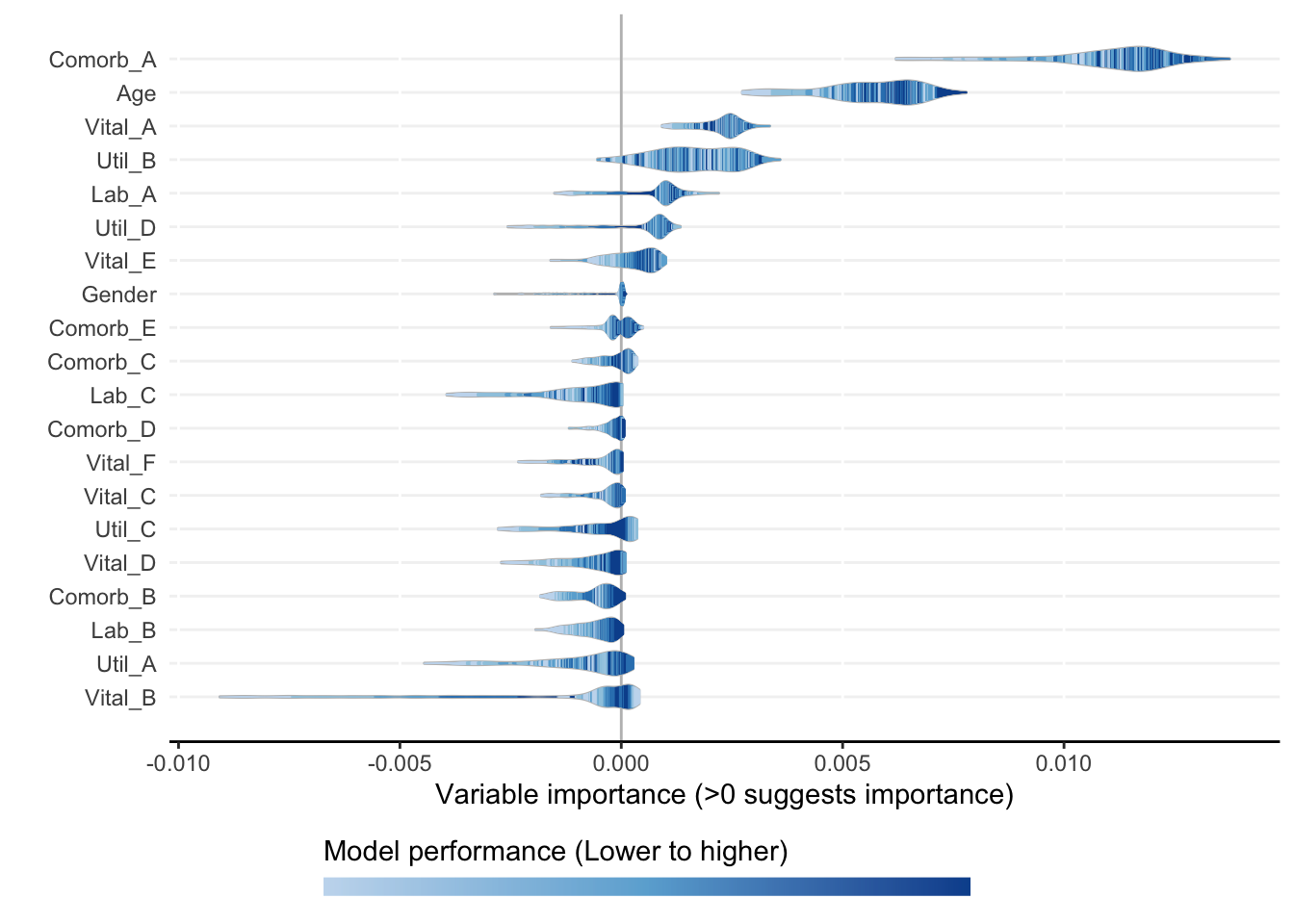
Specifically, as demonstrated in a recent clinical application, we use ShapleyVIC to analyse the importance of all candidate variables in the simulated dataset, exclude variables that have non-significant contribution to prediction, and apply the stepwise variable selection (starting with all significant contributors) to build sparse regression models for prediction.
Important
Although the outcome in this dataset is ordinal with 3 ordered categories, for demonstrative purpose we consider it as a continuous outcome in this chapter.
The previous chapter demonstrates how to analyse the same outcome as an ordinal variable.
In real-life clinical applications, users should take into consideration the nature of the outcome when choosing an analysis approach.
6.1 [R] Prepare data
This part of the workflow is implemented in R.
6.1.1 Load data
Load sample_data_ordinal from the AutoScore package.
Variable label is a simulated outcome label with 3 ordered categories.
Among the 20 predictor variables, Gender, Util_A and the 5 comorbidity variables (Comorb_A to Comorb_E) are categorical, and the rest are continuous.
library(AutoScore)library(dplyr)
Attaching package: 'dplyr'
The following objects are masked from 'package:stats':

    filter, lag
The following objects are masked from 'package:base':

    intersect, setdiff, setequal, union
 label          Age            Gender            Util_A          Util_B
 1:16360   Min.   : 18.00   FEMALE:10137   P1       : 3750   Min.   : 0.0000
 2: 2449   1st Qu.: 50.00   MALE  : 9863   P2       :11307   1st Qu.: 0.0000
 3: 1191   Median : 64.00                  P3 and P4: 4943   Median : 0.0000
           Mean   : 61.68                                    Mean   : 0.9267
           3rd Qu.: 76.00                                    3rd Qu.: 1.0000
           Max.   :109.00                                    Max.   :42.0000
     Util_C            Util_D         Comorb_A  Comorb_B  Comorb_C  Comorb_D
 Min.   :  0.000   Min.   : 0.09806   0:18445   0:17401   0:19474   0:18113
 1st Qu.:  0.000   1st Qu.: 1.52819   1: 1555   1: 2599   1:  526   1: 1887
 Median :  0.600   Median : 2.46306
 Mean   :  3.535   Mean   : 2.76030
 3rd Qu.:  3.970   3rd Qu.: 3.61472
 Max.   :293.680   Max.   :23.39056
 Comorb_E      Lab_A            Lab_B           Lab_C          Vital_A
 0:19690   Min.   :  16.0   Min.   :1.500   Min.   :102.0   Min.   :  0.00
 1:  310   1st Qu.:  66.0   1st Qu.:3.800   1st Qu.:133.0   1st Qu.: 70.00
           Median :  83.0   Median :4.100   Median :136.0   Median : 81.00
           Mean   : 146.9   Mean   :4.155   Mean   :135.2   Mean   : 82.67
           3rd Qu.: 115.0   3rd Qu.:4.400   3rd Qu.:138.0   3rd Qu.: 93.00
           Max.   :3534.0   Max.   :8.800   Max.   :170.0   Max.   :197.00
    Vital_B         Vital_C          Vital_D          Vital_E
 Min.   : 1.00   Min.   :  0.00   Min.   :  5.00   Min.   :  0.0
 1st Qu.:17.00   1st Qu.: 97.00   1st Qu.: 62.00   1st Qu.:116.0
 Median :18.00   Median : 98.00   Median : 70.00   Median :131.0
 Mean   :17.86   Mean   : 97.96   Mean   : 71.23   Mean   :133.5
 3rd Qu.:18.00   3rd Qu.: 99.00   3rd Qu.: 79.00   3rd Qu.:148.0
 Max.   :48.00   Max.   :100.00   Max.   :180.00   Max.   :262.0
    Vital_F
 Min.   : 2.30
 1st Qu.:21.10
 Median :23.00
 Mean   :22.82
 3rd Qu.:24.80
 Max.   :44.30
6.1.2 Prepare training, validation, and test datasets
Given large sample size (n=20000), split the data into training (70%), validation (10%) and test (20%) sets for regression model development.
For convenience, we reuse the stratified data split step from the previous chapter, but convert the outcome (“label”) to continuous.
set.seed(4)out_split <-split_data(data = sample_data_ordinal, ratio =c(0.7, 0.1, 0.2), strat_by_label =TRUE)train_set <- out_split$train_set# For this demo, convert the outcome ("label") to continuoustrain_set$label <-as.numeric(train_set$label)dim(train_set)
[1] 14000 21
validation_set <- out_split$validation_set# For this demo, convert the outcome ("label") to continuousvalidation_set$label <-as.numeric(validation_set$label)dim(validation_set)
[1] 2000 21
test_set <- out_split$test_set# For this demo, convert the outcome ("label") to continuoustest_set$label <-as.numeric(test_set$label)dim(test_set)
[1] 4000 21
Prepare cont_output for ShapleyVIC, using train_set as training set and validation_set as the explanation data.
Important
As detailed in Chapter 1, check for and handle data issues before applying ShapleyVIC. This demo uses data as-is because it is simulated clean data.
In this example the validation_set has 2000 samples, which is a reasonable sample size to be used as the explanation data. In cases with larger sample sizes, users should use a smaller subset as the explanation data (see Chapter 1 for detail).
from ShapleyVIC import computem_svic = compute.compute_shapley_vic( model_obj=model_object, x_expl=dat_expl.drop(columns=[y_name]), y_expl=dat_expl[y_name], n_cores=20, # running on a PC with 40 logical processors threshold=0.05)
Note
For users’ reference, the command above took approximately 24 hours on a PC (Windows 10 Education; Intel(R) Xeon(R) Silver 4210 CPU @ 2.20GHz 2.19GHz (2 processors); 128GB RAM).
Starting with a model that include all variables above, develop a sparse regression model using AIC-based stepwise selection (implemented by the MASS package).
# Model with all ShapleyVIC-selected variables:m_svic_all <-lm(label ~ ., data = train_set[, c("label", vars_svic)])summary(m_svic_all)
Call:
lm(formula = label ~ ., data = train_set[, c("label", vars_svic)])

Residuals:
     Min       1Q   Median       3Q      Max
-1.59070 -0.24560 -0.17416 -0.06995  1.98002

Coefficients:
             Estimate Std. Error t value Pr(>|t|)
(Intercept) 0.7564288  0.0268424  28.180  < 2e-16 ***
Comorb_A1   0.4327596  0.0165608  26.131  < 2e-16 ***
Age         0.0036084  0.0002453  14.707  < 2e-16 ***
Vital_A     0.0021720  0.0002606   8.335  < 2e-16 ***
Util_B      0.0370323  0.0020596  17.980  < 2e-16 ***
Lab_A       0.0001014  0.0000225   4.507 6.63e-06 ***
---
Signif. codes:  0 '***' 0.001 '**' 0.01 '*' 0.05 '.' 0.1 ' ' 1

Residual standard error: 0.5258 on 13994 degrees of freedom
Multiple R-squared:  0.0861,    Adjusted R-squared:  0.08577
F-statistic: 263.7 on 5 and 13994 DF,  p-value: < 2.2e-16
# Backward selection:library(MASS)
Attaching package: 'MASS'
The following object is masked from 'package:dplyr':

    select
ShapleyVIC-assisted backward selection developed a more parsimonious model (with 5 variables) than conventional backward selection (with 9 variables) without significantly impairing performance.
compute_mse <-function(y, y_pred) {mean((y - y_pred) ^2)}# Mean squared error (MSE) of the two models on test set:c(ShapleyVIC_assisted_backward_selection =compute_mse(y = test_set$label, y_pred =predict(m_svic, newdata = test_set)),Conventional_backward_selection =compute_mse(y = test_set$label, y_pred =predict(m_back, newdata = test_set)))