As introduced in the ShapleyVIC paper, this method can be applied to regression models beyond the logistic regression. This chapter provides a reproducible example to demonstrate its application for ordinal outcomes using a simulated dataset with ordinal outcome from the AutoScore package. The data is described in detail in the AutoScore Guidebook.
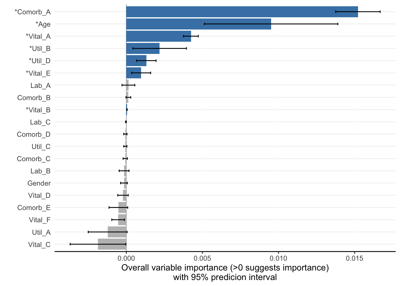
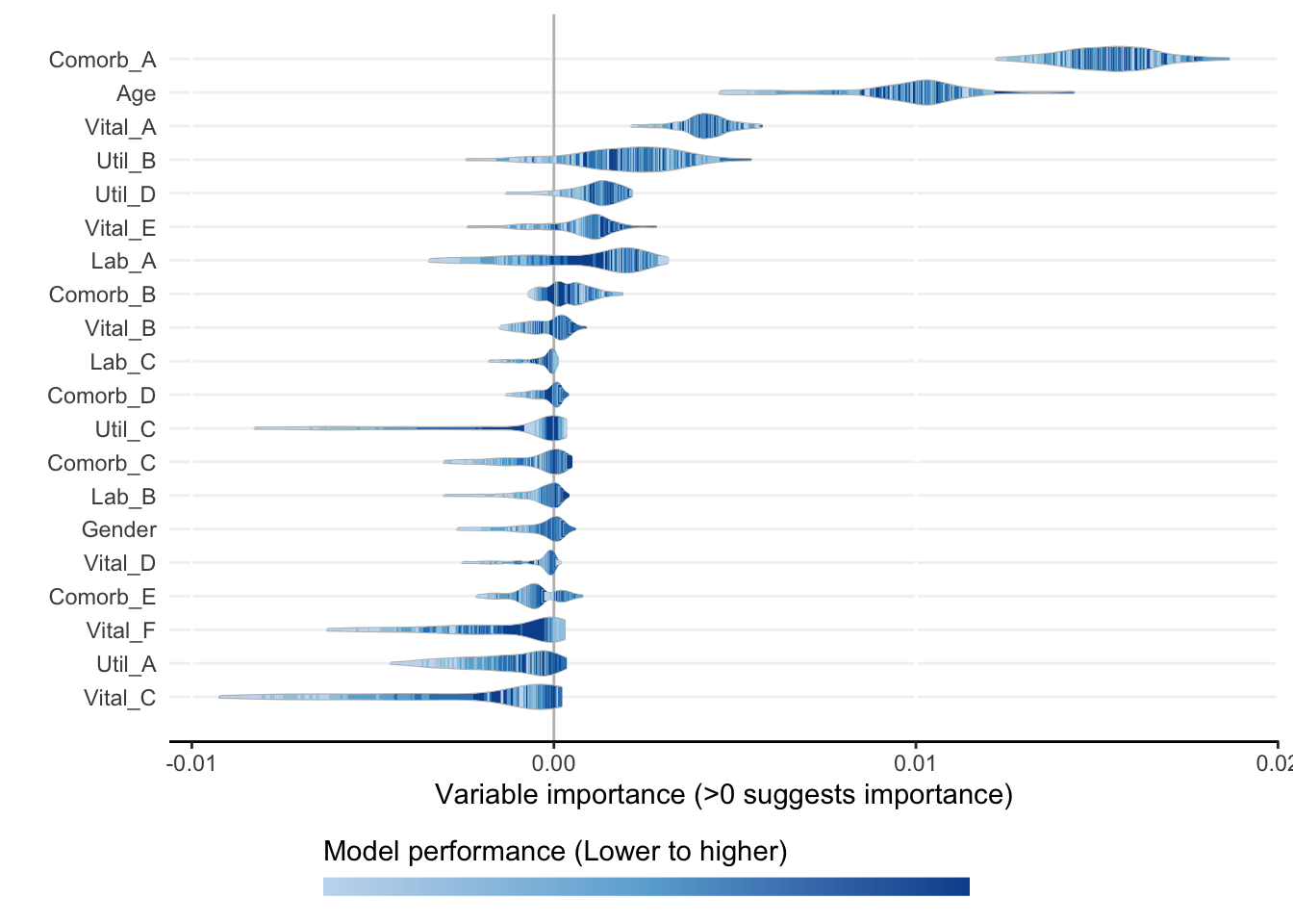
Specifically, as demonstrated in a recent clinical application, we use ShapleyVIC to analyse the importance of all candidate variables in the simulated dataset, exclude variables that have non-significant contribution to prediction, and apply the stepwise variable selection (starting with all significant contributors) to build sparse regression models for prediction.
5.1 [R] Prepare data
This part of the workflow is implemented in R.
5.1.1 Load data
Load sample_data_ordinal from the AutoScore package.
Variable label is a simulated outcome label with 3 ordered categories.
Among the 20 predictor variables, Gender, Util_A and the 5 comorbidity variables (Comorb_A to Comorb_E) are categorical, and the rest are continuous.
library(AutoScore)library(dplyr)
Attaching package: 'dplyr'
The following objects are masked from 'package:stats':

    filter, lag
The following objects are masked from 'package:base':

    intersect, setdiff, setequal, union
Prepare ord_output for ShapleyVIC, using train_set as training set and validation_set as the explanation data.
Important
As detailed in Chapter 1, check for and handle data issues before applying ShapleyVIC. This demo uses data as-is because it is simulated clean data.
In this example the validation_set has 2000 samples, which is a reasonable sample size to be used as the explanation data. In cases with larger sample sizes, users should use a smaller subset as the explanation data (see Chapter 1 for detail).
from ShapleyVIC import computem_svic = compute.compute_shapley_vic( model_obj=model_object, x_expl=dat_expl.drop(columns=[y_name]), y_expl=dat_expl[y_name], n_cores=20, # running on a PC with 40 logical processors threshold=0.05)
Note
For users’ reference, the command above took approximately 18 hours on a PC (Windows 10 Education; Intel(R) Xeon(R) Silver 4210 CPU @ 2.20GHz 2.19GHz (2 processors); 128GB RAM).
Starting with a model that include all variables above, develop a sparse regression model using AIC-based stepwise selection (implemented by the MASS package).
Using the ordinal package to develop ordinal regression models, more specifically cumulative link model (CLM) with the logit link. See the ordinal package for detailed usage.
# Model with all ShapleyVIC-selected variables:library(ordinal)
Attaching package: 'ordinal'
The following object is masked from 'package:dplyr':

    slice
m_svic_all <-clm(label ~ ., data = train_set[, c("label", vars_svic)])summary(m_svic_all)
ShapleyVIC-assisted backward selection developed a more parsimonious model (with 6 variables) than conventional backward selection (with 10 variables) without significantly impairing performance.
# Performance of model from ShapleyVIC-assisted backward selection on test set:fx_svic <-model.matrix(~ ., data = test_set[, x_svic])[, -1] %*% m_svic$betaprint_performance_ordinal(label = test_set$label, score =as.numeric(fx_svic), n_boot =100, report_cindex =TRUE)
# Performance of model from conventional backward selection on test set:fx_back <-model.matrix(~ ., data = test_set[, x_back])[, -1] %*% m_back$betaprint_performance_ordinal(label = test_set$label, score =as.numeric(fx_back), n_boot =100, report_cindex =TRUE)